Rendering check

Sample equations, code, a figure, and the lesson constructs, used to check how the site renders.

This page is not a lesson. It holds one sample of each kind of content a lesson uses, so that rendering can be checked in every browser engine and by the automated checks of the site.

Equations

Inline: the period of a pendulum of length $\ell$ at small amplitude is $T = 2\pi\sqrt{\ell / g}$.

Display, with a fraction, a root, and Greek letters:

$$x(t) = A\, e^{-\gamma t} \cos(\omega t), \qquad \omega = \sqrt{\omega_0^{2} - \gamma^{2}}.$$

Aligned steps:

$$\begin{aligned} \frac{\mathrm{d}E}{\mathrm{d}t} &= m v \frac{\mathrm{d}v}{\mathrm{d}t} + k x \frac{\mathrm{d}x}{\mathrm{d}t} \\ &= v \left( m \frac{\mathrm{d}v}{\mathrm{d}t} + k x \right) \\ &= 0. \end{aligned}$$

An integral, a sum, and a matrix:

$$W = \int_{x_0}^{x_1} F(x)\, \mathrm{d}x, \qquad p = \sum_{i=1}^{N} m_i v_i, \qquad \begin{pmatrix} x_{n+1} \\ v_{n+1} \end{pmatrix} = \begin{pmatrix} 1 & \Delta t \\ -\omega^{2} \Delta t & 1 \end{pmatrix} \begin{pmatrix} x_n \\ v_n \end{pmatrix}.$$

Code

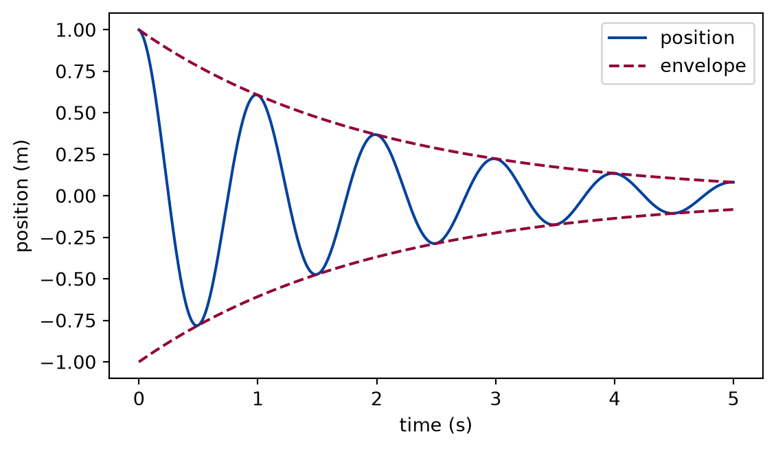
The cell below is executed when the site is built. It imports the function from the pbc package of the repository, so the listing and the output cannot drift apart.

import numpy as np

from pbc.sample import damped_oscillation

t = np.linspace(0.0, 2.0, 5)
for time, position in zip(t, damped_oscillation(t), strict=True):
    print(f"t = {time:.1f} s   x = {position:+.4f} m")

t = 0.0 s   x = +1.0000 m
t = 0.5 s   x = -0.7788 m
t = 1.0 s   x = +0.6065 m
t = 1.5 s   x = -0.4724 m
t = 2.0 s   x = +0.3679 m

Figure

import matplotlib.pyplot as plt
from pbc.authoring import FIGURE_COLOURS

t = np.linspace(0.0, 5.0, 1001)
envelope = np.exp(-0.5 * t)

fig, ax = plt.subplots(figsize=(6.4, 3.6))
ax.plot(t, damped_oscillation(t), color=FIGURE_COLOURS[0], label="position")
ax.plot(t, envelope, color=FIGURE_COLOURS[1], linestyle="--", label="envelope")
ax.plot(t, -envelope, color=FIGURE_COLOURS[1], linestyle="--")
ax.set_xlabel("time (s)")
ax.set_ylabel("position (m)")
ax.legend()
plt.show()

Figure 1: simulated A damped oscillation and its envelope.

Measured data

The pattern of a measured-data lab (docs/authoring.md, “Measured data”): the data card of the dataset, rendered from its card, and a figure made from the committed sample whose status the build checks against that card.

Data card

Dataset

NPL on-wafer S-parameters of attenuators and loads up to 220 GHz

Source

https://zenodo.org/records/22658069, DOI 10.5281/zenodo.22658069, Liam Ausden, Nick Ridler, Andrej Rumiantsev, Jon Martens, Xiaobang Shang (National Physical Laboratory, MPI Corporation, Anritsu); Zenodo record 22658069, published 2025-09-25 (no version number)

Licence

CC-BY-4.0

Attribution

Creators as above, 'Dataset for the Comparison of Broadband Single-Sweep and Conventional Banded System On-Wafer S-Parameter Measurements up to 220 GHz', Zenodo, doi 10.5281/zenodo.22658069, CC BY 4.0; supports the ARFTG 2025 paper doi 10.1109/ARFTG65332.2025.11168146.

Calibration

Multiline TRL on-wafer calibration, applied by the creators ('_CORR'; readme.txt). The calibration standards and their uncertainty are described in the ARFTG paper, which this spike did not read; the files carry no uncertainty.

Masks

None: no missing values in the four sampled files.

Uncertainty

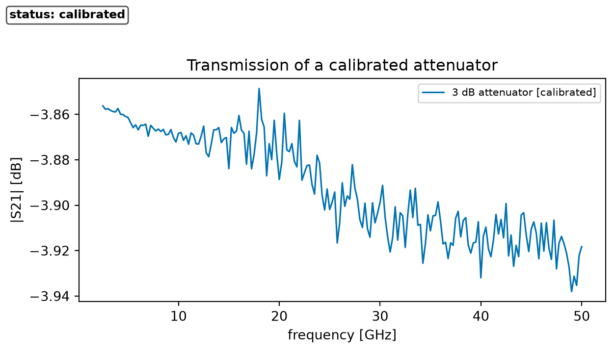
None in the files. The paper compares two instruments; this spike's cross-check shows the 3 dB pad's |S21| differing by at most 0.042 dB between the coaxial and the single-sweep file over 2.5-50 GHz.

Artifacts of the dataset NPL on-wafer S-parameters of attenuators and loads up to 220 GHz and the figure status each gives

Artifact	Type	Figure status	What it is
coaxial_*_CORR.s2p	calibrated-observation	calibrated	Coaxial-system VNA measurement of 3, 6, and 10 dB on-wafer attenuators, 2.5-50 GHz in 250 MHz steps; the '_CORR' files are calibrated with multiline TRL (readme.txt).
broadband_3dB_attenuator_0601_CORR.s2p	calibrated-observation	calibrated	Single-sweep broadband VNA measurement of the 3 dB attenuator, 2.5-220 GHz in 250 MHz steps, multiline-TRL calibrated.

A sample is committed in data/samples/npl-onwafer-sparameters/; the figures on this page are made from it.

The full data: ./scripts/fetch-data.sh npl-onwafer-sparameters downloads it into data/downloads/ and checks its digest. The site build and the checks never download anything.

No-LLM path. Everything on this page, the figures included, is reproduced from the files named here by the code of the page, with no language model and no account. An agent may help you explore the data; what it says is never data.

from pbc.data import SAMPLES_DIR
from pbc.data.adapters import transmission_series
from pbc.data.plotting import series_with_band
from pbc.data.touchstone import read_touchstone

network = read_touchstone(
    SAMPLES_DIR / "npl-onwafer-sparameters" / "coaxial_3dB_attenuator_0601_CORR.s2p"
)
fig, ax = series_with_band(transmission_series(network), "3 dB attenuator", figsize=(6.4, 3.6))
ax.set_title("Transmission of a calibrated attenuator")
plt.show()

Figure 2: calibrated Transmission of a calibrated 3 dB attenuator against frequency.

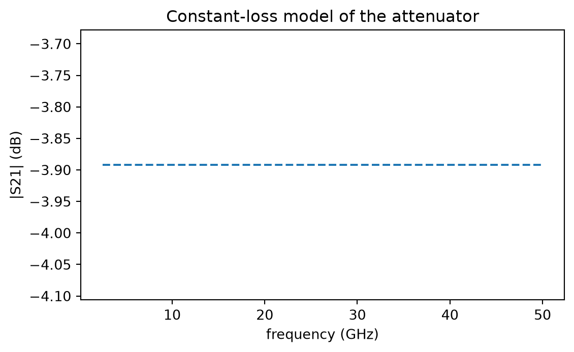
A figure of a model fitted to the dataset shows no data; it is simulated and names the dataset it was fitted to:

import numpy as np

measured = transmission_series(network)
loss = float(np.mean(measured.y))

fig, ax = plt.subplots(figsize=(6.4, 3.6))
ax.plot(measured.x, np.full_like(measured.x, loss), linestyle="--")
ax.set_xlabel(f"{measured.x_name} ({measured.x_unit})")
ax.set_ylabel(f"{measured.y_name} ({measured.y_unit})")
ax.set_title("Constant-loss model of the attenuator")
plt.show()

Figure 3: simulated A constant-loss model fitted to the transmission of the attenuator.

Lesson constructs

These are the constructs of the lesson format, one of each.

A listing included by reference from the package:

def damped_oscillation(
    t: ArrayLike,
    *,
    amplitude: float = 1.0,
    decay_rate: float = 0.5,
    angular_frequency: float = 2.0 * np.pi,
) -> NDArray[np.float64]:
    """Return ``amplitude * exp(-decay_rate * t) * cos(angular_frequency * t)``.

    ``t`` may be a scalar or an array; the result has the shape of ``t``.
    A negative ``decay_rate`` would describe a growing oscillation and is
    rejected.
    """
    if decay_rate < 0:
        raise ValueError(f"decay_rate must be non-negative, got {decay_rate}")
    time = np.asarray(t, dtype=np.float64)
    return amplitude * np.exp(-decay_rate * time) * np.cos(angular_frequency * time)

src/pbc/sample.py, lines 12 to 28, read from the repository when this page was built.

Material that the build did not run or check, as a block and inside a sentence:

Not verified. The build of this site did not run or check the material in this box.

position = damped_oscillation(time)  # a listing nothing executed

The oscillation loses about 39 percent (not verified) of its amplitude per second.

An exercise with a solution that opens without a script:

Exercise 1. What is the position at $t = 0$?

Solution to exercise 1

The amplitude, because $\cos 0 = 1$ and $e^{0} = 1$: 1.0 m.

A solution can hold material that the build did not run:

Not verified. The build of this site did not run or check the material in this box.

damped_oscillation(0.0)  # a listing nothing executed

Design components

One sample of each component of the visual system (docs/authoring.md, “Visual design”). The figure above shows the figure status in its caption.

What you’ll learn

• To read a claim label.
• To tell a measured figure from a simulated one.

Assumptions

• The oscillator is linear.
• Friction is proportional to speed.

Each claim type has its own label: observational, experimentally supported, numerically verified, and formal theorem.

The amplitude falls by the same factor every second.

Each figure status has its own label: measured calibrated processed simulated conceptual

Amplitude after whole periods.

Periods	Amplitude (m)	Error (m)
1	0.6065	0.0012
2	0.3679	0.0021

amplitude = initial * math.exp(-rate * time)

1. The amplitude decays exponentially.
2. The rate has the unit of one over a second.

Go deeper

• An optional reading, with a short reason to visit it.

Self-check. Why does the amplitude, and not the period, shrink?

Hint 1 of 1 for the self-check

Compare the two lengths of the motion.

With scripts, you can record in this browser that you answered this question.

Solution to the self-check

Friction removes energy, and the period depends on the stiffness and the mass.

1. Sample lesson

   One sentence about the lesson.

   Introductory, level 1 of 3

   • Simulation
   Details

   Outcomes and prerequisites.

2. M9 A planned lesson (planned, not published)

Kinematics, then Newton's laws, then the harmonic oscillator.

A sample attribution line.