Learning path

The lessons of the site by course and by method, with their difficulty and prerequisites.

Choose a physics course

Every lesson belongs to one physics course. Each course teaches by three activities: construct the physics as a program you can run and check, investigate it against measurements and with experiments that an AI agent helps to run, and verify the result, by tests, by independent checks, or by a machine-checked proof in Lean. Open a course below to see its lessons in teaching order, each with one preview and its level. Each lesson names the lessons it builds on and says what you will be able to do after it. Read a course from its first lesson, follow one method across courses, or start with any lesson whose prerequisites you have.

This page is generated from the lessons when the site is built. A course appears once it has a lesson, and a planned lesson is shown as planned. Methods and paths further down list the same lessons as links.

Courses

A lesson belongs to one course. Open a course to see its lessons in the teaching order of the reference curriculum. A planned lesson is not published: it has no page, and it is not counted.

With scripts, this place offers filters by course, method, difficulty, and publication state. Without them, the links above take you to each course, path, and method.

4 further courses have no lesson yet and are planned, so they are not shown as courses here: Fluid dynamics, Quantum physics, Astrophysics, cosmology, and relativity, and Condensed matter and materials physics.

Classical mechanics

Preview, simulated: Line plot of height in metres against time in seconds. The exact motion is a parabola: the ball rises, peaks halfway through the plotted time, and comes back down almost to its starting height. The explicit Euler points start on the parabola and then lie above it, by a distance that grows steadily with time.

Mechanics with numerical simulation: a model and its assumptions, a short program that steps it forward in time, and a comparison with what theory predicts. The core lessons are the mechanics lessons; the extensions repeat the course's results with an agent, with many agents, and with a proof.

28 published lessons, 4 planned.

Start with Kinematics as a program

Lessons of Classical mechanics (28 published)

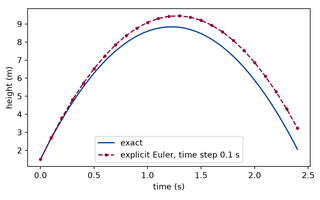
Kinematics as a program
Motion along a line under a known acceleration, written as a state and an update rule, and checked against the exact solution.
Introductory, level 1 of 3
- Simulation
Details of Kinematics as a program
Course
Classical mechanics
Slot
M1, Kinematics as a program
Methods
Simulation
Level
Introductory, level 1 of 3
What you build
Motion along a line under a known acceleration, written as a state and an update rule, and checked against the exact solution.
What you’ll learn
- Write motion along a line as a state and an update rule
- Check a simulation against the exact solution for constant acceleration
- Measure how the error of Euler stepping shrinks with the time step
Prerequisites
none on this site. Also assumed: Calculus: derivatives, integrals, and Taylor expansion to second order; Python: functions, dataclasses, and NumPy arrays; Logarithms: the base-2 logarithm, and reading a log-log plot.
Related
Proving what the simulation showed
On your machine
Run this experiment
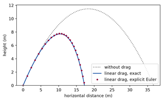
Newton’s laws as a first-order system
Forces as functions of the state, Newton's second law as a stepper that the rest of the course reuses, and a fall with linear drag checked against its exact solution.
Intermediate, level 2 of 3
- Simulation
Details of Newton’s laws as a first-order system
Course
Classical mechanics
Slot
M2, Newton's laws
Methods
Simulation
Level
Intermediate, level 2 of 3
What you build
Forces as functions of the state, Newton's second law as a stepper that the rest of the course reuses, and a fall with linear drag checked against its exact solution.
What you’ll learn
- Express a force as a function of the state and step Newton's second law
- Reuse one stepper for every system of the course
- Check a fall with linear drag against its exact solution
Prerequisites
Kinematics as a program. Also assumed: Calculus: first-order linear differential equations and the exponential function; Vectors: components, addition, and scaling.
Related
none
On your machine
Run this experiment
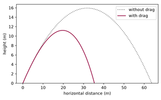
Projectile motion with quadratic drag
A thrown ball with drag that grows with the square of its speed has no closed-form motion, so the simulation is validated by its limiting cases and by convergence, and then used to find the range against the launch angle.
Intermediate, level 2 of 3
- Simulation
- AI extensions
Details of Projectile motion with quadratic drag
Course
Classical mechanics
Slot
M3, Projectile motion with drag
Methods
Simulation
Level
Intermediate, level 2 of 3
What you build
A thrown ball with drag that grows with the square of its speed has no closed-form motion, so the simulation is validated by its limiting cases and by convergence, and then used to find the range against the launch angle.
What you’ll learn
- Validate a simulation without an exact solution by limiting cases and convergence
- Read the order of convergence from a log-log plot
- Find the launch angle of greatest range with and without drag
Prerequisites
Newton’s laws as a first-order system. Also assumed: Trigonometry: the components of a vector at an angle; Logarithms: reading a log-log plot.
Related
An agent runs an experiment
On your machine
Run this experiment
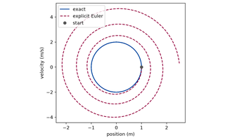
The harmonic oscillator
A mass on a spring as the test system of the course: its exact motion, its orbit in phase space, and the proof from the update rule that explicit Euler multiplies its energy by the same factor at every step.
Intermediate, level 2 of 3
- Simulation
Details of The harmonic oscillator
Course
Classical mechanics
Slot
M4, Harmonic oscillator
Methods
Simulation
Level
Intermediate, level 2 of 3
What you build
A mass on a spring as the test system of the course: its exact motion, its orbit in phase space, and the proof from the update rule that explicit Euler multiplies its energy by the same factor at every step.
What you’ll learn
- Solve the mass on a spring exactly and draw its orbit in phase space
- Show from the update rule that explicit Euler multiplies the energy by a fixed factor each step
- Use the oscillator as the test system for a stepping method
Prerequisites
Newton’s laws as a first-order system. Also assumed: Calculus: the derivatives of sine and cosine, and checking a solution by substitution; Logarithms: the natural logarithm and the exponential of a small number.
Related
Proving what the simulation showed
On your machine
Run this experiment
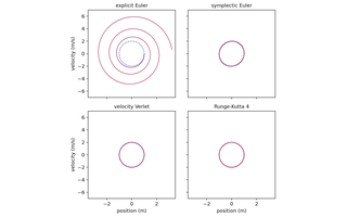
Numerical integrators
Explicit Euler, symplectic Euler, velocity Verlet, and Runge-Kutta 4 behind one stepping interface, compared on the harmonic oscillator for accuracy, energy behaviour, and cost, so that a later simulation can choose its method for what it has to be trusted for.
Intermediate, level 2 of 3
- Simulation
Details of Numerical integrators
Course
Classical mechanics
Slot
M5, Numerical integrators
Methods
Simulation
Level
Intermediate, level 2 of 3
What you build
Explicit Euler, symplectic Euler, velocity Verlet, and Runge-Kutta 4 behind one stepping interface, compared on the harmonic oscillator for accuracy, energy behaviour, and cost, so that a later simulation can choose its method for what it has to be trusted for.
What you’ll learn
- Step a system with explicit Euler, symplectic Euler, velocity Verlet, and Runge-Kutta 4 behind one interface
- Compare integrators for accuracy, energy behaviour, and cost
- Choose an integrator for what a simulation has to be trusted for
Prerequisites
The harmonic oscillator. Also assumed: Complex numbers: modulus, argument, and the exponential of an imaginary number; Calculus: Taylor expansion to fourth order; Linear algebra: the determinant and the trace of a two-by-two matrix.
Related
What symplectic Euler conserves
On your machine
Run this experiment
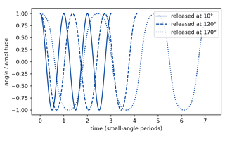
Energy conservation
Work, potential energy, and the pendulum at large amplitude, where no closed form gives the motion: the drift of the energy becomes the diagnostic of a simulation, with what it catches and what it does not.
Intermediate, level 2 of 3
- Simulation
Details of Energy conservation
Course
Classical mechanics
Slot
M6, Energy conservation
Methods
Simulation
Level
Intermediate, level 2 of 3
What you build
Work, potential energy, and the pendulum at large amplitude, where no closed form gives the motion: the drift of the energy becomes the diagnostic of a simulation, with what it catches and what it does not.
What you’ll learn
- Compute work and potential energy along a simulated motion
- Simulate the pendulum at large amplitude
- Use the drift of the energy as a diagnostic, and say what it does not catch
Prerequisites
Numerical integrators. Also assumed: Calculus: the chain rule, the integral of a function along a path, and Taylor expansion to second order; Trigonometry: the small-angle approximation of the sine; Vectors: the dot product, and the gradient of a function of the position.
Related
none
On your machine
Run this experiment
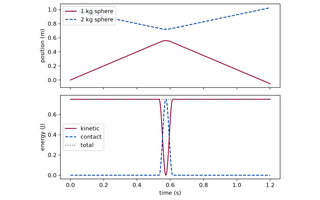
Momentum and collisions
Pairwise forces on the stepping interface, the total momentum that every integrator of the course then conserves to round-off, the centre of mass, and collisions as brief, strong forces whose outcome tends to the hard-sphere one.
Intermediate, level 2 of 3
- Simulation
Details of Momentum and collisions
Course
Classical mechanics
Slot
M7, Momentum and collisions
Methods
Simulation
Level
Intermediate, level 2 of 3
What you build
Pairwise forces on the stepping interface, the total momentum that every integrator of the course then conserves to round-off, the centre of mass, and collisions as brief, strong forces whose outcome tends to the hard-sphere one.
What you’ll learn
- Write pairwise forces on the stepping interface
- Check that the total momentum is conserved to round-off
- Model a collision as a brief strong force and compare it with the hard-sphere outcome
Prerequisites
Energy conservation. Also assumed: Vectors: components, the dot product, and the unit vector along a direction.
Related
Particles in a box, Momentum in a collision, proved
On your machine
Run this experiment
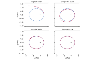
The Kepler orbit
The physics capstone of the mechanics course: two bodies under gravity reduced to one, the energy and the angular momentum that fix the ellipse, the exact orbit to measure against, and what each integrator does to a thousand orbits, with every tool of the earlier lessons reused.
Advanced, level 3 of 3
- Simulation
Details of The Kepler orbit
Course
Classical mechanics
Slot
M8, Kepler orbits
Methods
Simulation
Level
Advanced, level 3 of 3
What you build
The physics capstone of the mechanics course: two bodies under gravity reduced to one, the energy and the angular momentum that fix the ellipse, the exact orbit to measure against, and what each integrator does to a thousand orbits, with every tool of the earlier lessons reused.
What you’ll learn
- Reduce two bodies under gravity to one
- Derive the ellipse, its size, and its period from the energy and the angular momentum
- Compare each integrator with the exact orbit over a thousand orbits
Prerequisites
Energy conservation, Momentum and collisions. Also assumed: Vectors: the cross product in three dimensions, and the identity a × (b × c) = b (a·c) − c (a·b); Geometry: the ellipse, its foci, semi-major axis, and eccentricity; Numerical methods: the Newton iteration for the root of an equation.
Related
Gravitational-wave strain lab
On your machine
Run this experiment
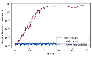
Double pendulum and chaos
Two rods hung from each other: a motion that is regular at small angles and chaotic at large ones, told apart by how fast two nearly identical starts separate, and measured by an estimate of the Lyapunov exponent that is checked against its expected sign in both regimes.
Advanced, level 3 of 3
- Simulation
Details of Double pendulum and chaos
Course
Classical mechanics
Slot
M9, Double pendulum and chaos
Methods
Simulation
Level
Advanced, level 3 of 3
What you build
Two rods hung from each other: a motion that is regular at small angles and chaotic at large ones, told apart by how fast two nearly identical starts separate, and measured by an estimate of the Lyapunov exponent that is checked against its expected sign in both regimes.
What you’ll learn
- Simulate the double pendulum and check it against its small-oscillation modes and its energy
- Measure how two nearly identical starts separate, in a regular and in a chaotic motion
- Estimate the largest Lyapunov exponent and say what its sign means
- State how long a chaotic motion can be predicted, and what a finer step does and does not change
Prerequisites
Energy conservation, Numerical integrators. Also assumed: Calculus: the chain rule, and the exponential function as the solution of a rate proportional to the amount; Trigonometry: the sine and cosine of a difference of angles; Logarithms: the natural logarithm of a ratio, and its use to read a growth rate from a straight line on a logarithmic axis; Linear algebra: the Euclidean norm of a vector.
Related
Lagrangian mechanics
On your machine
Run this experiment
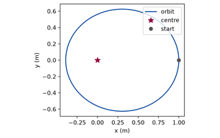
Lagrangian mechanics
The equations of motion of a constrained or coupled system from one function, the kinetic minus the potential energy, simulated and checked against the Newtonian form for the pendulum, two coupled springs, a planet, and the equations of the double pendulum.
Advanced, level 3 of 3
- Simulation
Details of Lagrangian mechanics
Course
Classical mechanics
Slot
M10, Lagrangian mechanics
Methods
Simulation
Level
Advanced, level 3 of 3
What you build
The equations of motion of a constrained or coupled system from one function, the kinetic minus the potential energy, simulated and checked against the Newtonian form for the pendulum, two coupled springs, a planet, and the equations of the double pendulum.
What you’ll learn
- Write the Lagrangian of a system in coordinates that fit its constraints
- Obtain and simulate its equations of motion from the Euler-Lagrange equations
- Check the equations against the Newtonian form in cases with a closed form
- Read a conserved momentum off a coordinate that the Lagrangian does not contain
Prerequisites
Energy conservation, Double pendulum and chaos. Also assumed: Calculus: partial derivatives, and the chain rule for a function of several variables; Linear algebra: solving a system of linear equations written with a matrix; Trigonometry: the sine and cosine, and polar coordinates.
Related
Hamiltonian mechanics
On your machine
Run this experiment
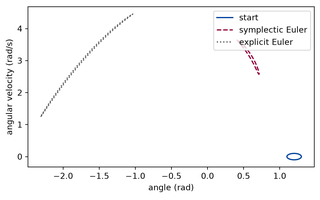
Hamiltonian mechanics
Phase space, Hamilton's equations from the Lagrangian, the area that a symplectic step preserves and the others do not, and the modified energy that such a step conserves, checked against the conserved quantities of the numerical-integrators lesson and of the Lean lesson on symplectic Euler.
Advanced, level 3 of 3
- Simulation
Details of Hamiltonian mechanics
Course
Classical mechanics
Slot
M11, Hamiltonian mechanics
Methods
Simulation
Level
Advanced, level 3 of 3
What you build
Phase space, Hamilton's equations from the Lagrangian, the area that a symplectic step preserves and the others do not, and the modified energy that such a step conserves, checked against the conserved quantities of the numerical-integrators lesson and of the Lean lesson on symplectic Euler.
What you’ll learn
- Obtain the Hamiltonian from a Lagrangian and write the motion as a flow in phase space
- Measure how a step of an integrator changes the area of a region of phase space
- Check that a symplectic method conserves its modified energy, on the oscillator and on the pendulum
- Choose between a symplectic and a higher-order method for a given length of run
Prerequisites
Lagrangian mechanics, Numerical integrators, What symplectic Euler conserves. Also assumed: Calculus: partial derivatives; Linear algebra: the determinant of a two-by-two matrix, and the matrix of derivatives of a map; Geometry: the area of a region bounded by a closed curve.
Related
none
On your machine
Run this experiment
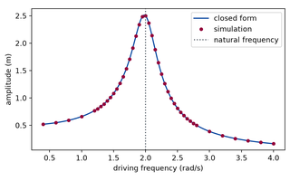
Resonance and driven oscillators
A damped oscillator pushed at a steady rhythm: the amplitude and phase that it settles into, the resonance curve with its peak and width, and a simulation of the whole curve validated against the analytic amplitude.
Intermediate, level 2 of 3
- Simulation
Details of Resonance and driven oscillators
Course
Classical mechanics
Slot
M12, Resonance and driven oscillators
Methods
Simulation
Level
Intermediate, level 2 of 3
What you build
A damped oscillator pushed at a steady rhythm: the amplitude and phase that it settles into, the resonance curve with its peak and width, and a simulation of the whole curve validated against the analytic amplitude.
What you’ll learn
- Write the damped, driven oscillator and its steady-state amplitude and phase
- Read the peak, the width, and the quality factor off a resonance curve
- Simulate the curve and validate it against the analytic amplitude, with the transient separated from the steady state
- Say how long a driven system takes to settle and why a larger quality factor takes longer
Prerequisites
The harmonic oscillator, Projectile motion with quadratic drag, Numerical integrators. Also assumed: Calculus: derivatives, and the maximum of a function found where its derivative is zero; Complex numbers: the exponential of an imaginary number, and the modulus and argument of a complex ratio; Trigonometry: the amplitude and phase of a sum of a sine and a cosine of the same frequency.
Related
none
On your machine
Run this experiment
M13 Many-body gravitation (planned, not published)
M14 Nonlinear dynamics and bifurcations (planned, not published)
M17 Rotational motion, torque, and angular momentum (planned, not published)
M15 Experimental: real pendulum or accelerometer data, measured-data lab (planned, not published)
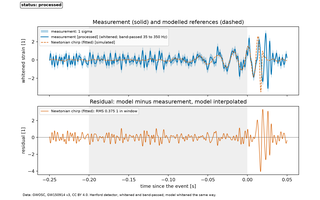
Gravitational-wave strain lab
From the Kepler orbit to a chirp: the calibrated strain of the two LIGO detectors around the first detected gravitational-wave event, whitened and compared with the Newtonian-order chirp of two bodies spiralling together, and what that comparison does and does not say about the masses.
Advanced, level 3 of 3
- Simulation
- Experimental data
Details of Gravitational-wave strain lab
Course
Classical mechanics
Slot
M16, Experimental: GW150914 gravitational-wave strain
Methods
Measured data, Simulation
Level
Advanced, level 3 of 3
What you build
From the Kepler orbit to a chirp: the calibrated strain of the two LIGO detectors around the first detected gravitational-wave event, whitened and compared with the Newtonian-order chirp of two bodies spiralling together, and what that comparison does and does not say about the masses.
What you’ll learn
- Derive the frequency and the rate of change of frequency of a shrinking circular orbit from Kepler's third law and an energy loss
- Read a measured strain through the processing it needs, saying at each step what was changed
- Fit the Newtonian chirp to the whitened strain, report the chirp mass with its uncertainty, and say what the model leaves out
Prerequisites
The Kepler orbit. Also assumed: Complex numbers: the discrete Fourier transform of a sampled signal, its spectrum, and what a window does to it; Statistics: a least-squares fit, the standard deviation of noise, and the chi-square of residuals.
Related
The chirp law, proved
Classification
Measured-data lab of Classical mechanics; the prerequisites above are what it builds on.
On your machine
Run this experiment
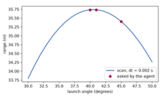
An agent runs an experiment
A language model designs and runs an experiment on the projectile simulation through a short, bounded list of tools, and CI checks the recorded run by recomputing every tool result without a model or a key.
Intermediate, level 2 of 3
- Simulation
- AI extensions
Details of An agent runs an experiment
Course
Classical mechanics
Slot
AI0, LLM agent designs a projectile experiment
Methods
Simulation, LLM agents
Level
Intermediate, level 2 of 3
What you build
A language model designs and runs an experiment on the projectile simulation through a short, bounded list of tools, and CI checks the recorded run by recomputing every tool result without a model or a key.
What you’ll learn
- Give a language model a short, bounded list of tools to run a simulation
- Read a recorded agent run as an experiment
- Recompute every tool result of a run without a model or a key
- Say what a replay does and does not show about an agent's conclusion
Prerequisites
Projectile motion with quadratic drag. Also assumed: Python: functions, dictionaries, and environment variables; Large language models: a program that continues a text.
Related
none
On your machine
Replay this experiment
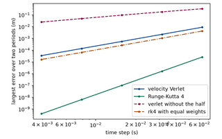
Verifying scientific code
How a piece of simulation code is shown to be right or wrong: independent tests from limits, conservation, and convergence, six deliberately faulty steppers that the tests must catch, and the written contract that says what a verifier checks, in what order, and with what evidence.
Advanced, level 3 of 3
- Simulation
Details of Verifying scientific code
Course
Classical mechanics
Slot
AI2, Scientific code verification and debugging
Methods
Simulation
Level
Advanced, level 3 of 3
What you build
How a piece of simulation code is shown to be right or wrong: independent tests from limits, conservation, and convergence, six deliberately faulty steppers that the tests must catch, and the written contract that says what a verifier checks, in what order, and with what evidence.
What you’ll learn
- Test a simulation against limits, conservation, and convergence with references independent of the code
- Catch a deliberately faulty stepper with a named test and explain why other tests miss it
- Evaluate a piece of code against a stated claim, with the evidence in a fixed form
Prerequisites
Numerical integrators, Energy conservation. Also assumed: Python: reading a short function and a unit test.
Related
none
On your machine
Run this experiment
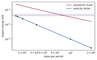
A counterexample hunter
A language model tries to refute two claims about integrators through a bounded list of simulations; the build recomputes every experiment and decides the verdict itself, so that only a recomputed counterexample counts as a result and a failed hunt is labelled inconclusive.
Advanced, level 3 of 3
- Simulation
- AI extensions
Details of A counterexample hunter
Course
Classical mechanics
Slot
AI3, Counterexample hunting
Methods
Simulation, LLM agents
Level
Advanced, level 3 of 3
What you build
A language model tries to refute two claims about integrators through a bounded list of simulations; the build recomputes every experiment and decides the verdict itself, so that only a recomputed counterexample counts as a result and a failed hunt is labelled inconclusive.
What you’ll learn
- State a falsifiable claim with a predicate and a budget of experiments
- Read a worked hunt and the verdict the build recomputed from it
- Explain why a failed hunt is inconclusive and not a proof
Prerequisites
An agent runs an experiment, Numerical integrators. Also assumed: Python: functions and dictionaries; Large language models: a program that continues a text.
Related
Verifying scientific code
On your machine
Replay this experiment
Three reviewers for one piece of code
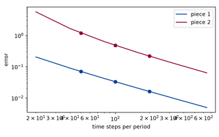
Three review agents, one for the physics, one for the numerical implementation, and one for the evidence, each with a short list of checks from the scientific validation contract, review a correct stepper and a faulty one; where they disagree, the build recomputes every check and the failed one stands.
Advanced, level 3 of 3
- Simulation
- AI extensions
Details of Three reviewers for one piece of code
Course
Classical mechanics
Slot
AI4, Multi-agent scientific review
Methods
Simulation, LLM agents
Level
Advanced, level 3 of 3
What you build
Three review agents, one for the physics, one for the numerical implementation, and one for the evidence, each with a short list of checks from the scientific validation contract, review a correct stepper and a faulty one; where they disagree, the build recomputes every check and the failed one stands.
What you’ll learn
- Give each of several review agents its own bounded list of checks over the same code
- Read a disagreement between reviewers as a difference in what each one checked
- Decide a review from recomputed check results, not from the words of a reviewer
Prerequisites
An agent runs an experiment, Verifying scientific code. Also assumed: Python: reading a short function and a dictionary.
Related
none
On your machine
Replay this experiment
Discovering a force law with controlled probes
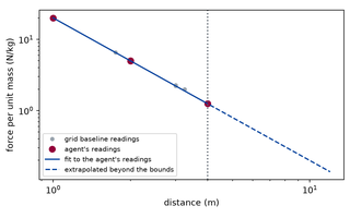
A language model probes a black box that pulls a test body toward a centre, one control at a time, and submits a force law; the build scores the claim on distances it could not probe and sets it beside three baselines that use no model.
Intermediate, level 2 of 3
- Simulation
- AI extensions
Details of Discovering a force law with controlled probes
Course
Classical mechanics
Slot
D1, Black-box physics: discovering force laws
Methods
Simulation, LLM agents
Level
Intermediate, level 2 of 3
What you build
A language model probes a black box that pulls a test body toward a centre, one control at a time, and submits a force law; the build scores the claim on distances it could not probe and sets it beside three baselines that use no model.
What you’ll learn
- Design controlled probes that separate the effect of each control on a force
- Read an exponent from the ratio of two forces at two distances, and say how the noise limits it
- Score a claimed law on settings outside the probed range, and compare it with baselines that use no model
- Say what a good score of a recorded run does and does not show about the agent
Prerequisites
An agent runs an experiment, Inverse physics: parameters from observations. Also assumed: Logarithms: the logarithm of a product and of a power; Large language models: a program that continues a text.
Related
none
On your machine
Replay this experiment
Full, partial, and no prior knowledge under one protocol
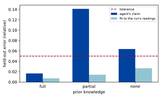
The same language model probes the same hidden spring three times, told the form of the law, only the names of its parameters, or nothing; the build scores the three claims on the same held-out settings and shows what the agent's own readings would have supported.
Advanced, level 3 of 3
- Simulation
- AI extensions
Details of Full, partial, and no prior knowledge under one protocol
Course
Classical mechanics
Slot
D2, Physics without prior knowledge
Methods
Simulation, LLM agents
Level
Advanced, level 3 of 3
What you build
The same language model probes the same hidden spring three times, told the form of the law, only the names of its parameters, or nothing; the build scores the three claims on the same held-out settings and shows what the agent's own readings would have supported.
What you’ll learn
- Set up a comparison of conditions in which only the prior knowledge differs, and check that it does
- Infer a spring's force law from the motion it causes, and say why late times constrain it most
- Separate what a run's readings support from what the agent concluded from them
- Explain why one run per condition cannot rank the conditions
Prerequisites
Discovering a force law with controlled probes, The harmonic oscillator. Also assumed: Trigonometry: the cosine and its period; Statistics: least squares and the chi-square of residuals.
Related
none
On your machine
Replay this experiment
Unlearning a familiar law: a modified force
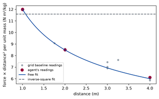
A language model probes a central force whose law is not the inverse square it knows; the build shows that the familiar law fails the readings, that a baseline without a model identifies the modified one, and reports the agent's claim exactly as it scored.
Advanced, level 3 of 3
- Simulation
- AI extensions
Details of Unlearning a familiar law: a modified force
Course
Classical mechanics
Slot
D3, Discovering modified physical laws
Methods
Simulation, LLM agents
Level
Advanced, level 3 of 3
What you build
A language model probes a central force whose law is not the inverse square it knows; the build shows that the familiar law fails the readings, that a baseline without a model identifies the modified one, and reports the agent's claim exactly as it scored.
What you’ll learn
- Test a familiar law against readings and reject it with a stated criterion
- Identify a modified exponent with a baseline that uses no model, and score it beyond the probed range
- Tell a fit that is consistent where it was probed from one that is right where it was not
- Report an agent's result as it scored, whether or not the baseline did better
Prerequisites
Discovering a force law with controlled probes, The Kepler orbit. Also assumed: Statistics: least squares and the chi-square of residuals; Logarithms: the logarithm of a product and of a power.
Related
none
On your machine
Replay this experiment
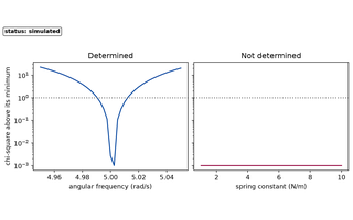
Inverse physics: parameters from observations
Fitting a model to observations to find its parameters: how to check a fit against known answers, how to state the uncertainty, how to see that the data cannot tell two parameters apart or that the model is wrong, and what that means for the chirp mass read from the gravitational-wave strain.
Advanced, level 3 of 3
- Simulation
- Experimental data
Details of Inverse physics: parameters from observations
Course
Classical mechanics
Slot
D6, Inverse physics: parameter discovery and uncertainty
Methods
Simulation, Measured data
Level
Advanced, level 3 of 3
What you build
Fitting a model to observations to find its parameters: how to check a fit against known answers, how to state the uncertainty, how to see that the data cannot tell two parameters apart or that the model is wrong, and what that means for the chirp mass read from the gravitational-wave strain.
What you’ll learn
- Check a fitting procedure on synthetic data of known parameters, and say what recovery, bias, and coverage of the stated interval mean
- Tell from a profile of the chi-square whether the data bound a parameter, and recognise two parameters that appear only as a combination
- List the reasons not to take a converged fit as evidence for its model
- State the uncertainty of a parameter fitted to measured data, with the scatter that an injection of a known signal shows
Prerequisites
The harmonic oscillator, Gravitational-wave strain lab. Also assumed: Statistics: least squares, the chi-square of residuals, and a standard error.
Related
none
On your machine
Run this experiment
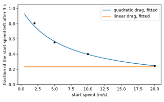
An agent that designs the measurements
A language model chooses where to measure the slowing of a sliding block so that two models of drag can be told apart, within a budget; the build scores the design, fits both models to the readings it recomputes, and types the conclusion only as far as those numbers support it.
Advanced, level 3 of 3
- Simulation
- AI extensions
Details of An agent that designs the measurements
Course
Classical mechanics
Slot
D9, Active experimental design
Methods
Simulation, LLM agents
Level
Advanced, level 3 of 3
What you build
A language model chooses where to measure the slowing of a sliding block so that two models of drag can be told apart, within a budget; the build scores the design, fits both models to the readings it recomputes, and types the conclusion only as far as those numbers support it.
What you’ll learn
- Say what makes a measurement useful for telling two models apart, and score a design before any reading exists
- Read a worked run of an agent that chooses its measurements, and the assessment the build recomputed from it
- Explain why measurements that fit one model better are not yet a result, and what an inconclusive design looks like
Prerequisites
A counterexample hunter, Inverse physics: parameters from observations. Also assumed: Statistics: least squares and the chi-square of residuals; Python: functions and dictionaries.
Related
none
On your machine
Replay this experiment
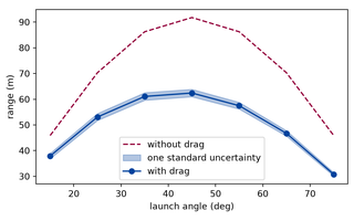
Automated analysis pipelines
One reusable workflow, a parameter sweep, a statistic with its uncertainty, a figure, and a report that the build regenerates and compares with a committed expectation, run on a simulated throw and on measured waves.
Intermediate, level 2 of 3
- Simulation
- Experimental data
Details of Automated analysis pipelines
Course
Classical mechanics
Slot
R1, Automated physics analysis pipelines
Methods
Simulation, Measured data
Level
Intermediate, level 2 of 3
What you build
One reusable workflow, a parameter sweep, a statistic with its uncertainty, a figure, and a report that the build regenerates and compares with a committed expectation, run on a simulated throw and on measured waves.
What you’ll learn
- Write an analysis as a function that a sweep, a repetition, and a report can all reuse
- Carry the uncertainty of an input to a result, and check that propagation with a seeded Monte Carlo run
- Tell the scatter of repetitions from the effect of an analysis choice, and report both
- Turn the numbers of an analysis into a report that a build compares with a committed expectation
Prerequisites
Projectile motion with quadratic drag. Also assumed: Statistics: the mean, the standard deviation, and the standard error of a mean.
Related
none
On your machine
Run this experiment
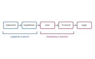
Proving what the simulation showed
Two results of the mechanics course stated and proved in Lean 4: the identity that links speed and distance under constant acceleration, and the factor by which one step of explicit Euler multiplies the energy of the harmonic oscillator, with the proofs compiled by CI and read from the repository.
Intermediate, level 2 of 3
Details of Proving what the simulation showed
Course
Classical mechanics
Slot
L1, Proving what the simulation showed
Methods
Formal proofs
Level
Intermediate, level 2 of 3
What you build
Two results of the mechanics course stated and proved in Lean 4: the identity that links speed and distance under constant acceleration, and the factor by which one step of explicit Euler multiplies the energy of the harmonic oscillator, with the proofs compiled by CI and read from the repository.
What you’ll learn
- State a result of the mechanics course as a theorem in Lean 4
- Read the proof of the identity between speed and distance under constant acceleration
- Read the proof of the factor by which one Euler step multiplies the energy of the oscillator
Prerequisites
Kinematics as a program, The harmonic oscillator. Also assumed: Algebra: expanding and factorising polynomials in several variables; Logic: reading a statement that says if these hypotheses hold, then this conclusion holds.
Related
none
On your machine
Check this proof
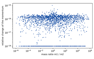
Momentum in a collision, proved
The collision rule of two hard spheres from the momentum lesson, stated in Lean 4, with a proof that it conserves the total momentum along every axis for every choice of masses, velocities, and direction.
Intermediate, level 2 of 3
Details of Momentum in a collision, proved
Course
Classical mechanics
Methods
Formal proofs
Level
Intermediate, level 2 of 3
What you build
The collision rule of two hard spheres from the momentum lesson, stated in Lean 4, with a proof that it conserves the total momentum along every axis for every choice of masses, velocities, and direction.
What you’ll learn
- State the collision rule of two hard spheres as a definition in Lean 4
- Read the proof that the rule conserves the total momentum along every axis
- Say which part of the momentum conservation seen in the simulation the theorem covers, and which it leaves out
Prerequisites
Momentum and collisions, Proving what the simulation showed. Also assumed: Vectors: components and the dot product.
Related
none
On your machine
Check this proof
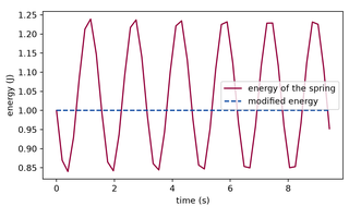
What symplectic Euler conserves
A modified energy that every step of symplectic Euler leaves exactly unchanged on the harmonic oscillator, stated and proved in Lean 4, with the step size under which it stays bounded, and the reason the energy of the method oscillates and does not grow.
Advanced, level 3 of 3
Details of What symplectic Euler conserves
Course
Classical mechanics
Methods
Formal proofs
Level
Advanced, level 3 of 3
What you build
A modified energy that every step of symplectic Euler leaves exactly unchanged on the harmonic oscillator, stated and proved in Lean 4, with the step size under which it stays bounded, and the reason the energy of the method oscillates and does not grow.
What you’ll learn
- State the modified energy of symplectic Euler and its conservation as theorems in Lean 4
- Read the proof by induction that the modified energy is the same after any number of steps
- Say what the theorem explains about the bounded energy seen in the simulation, and what it does not prove
Prerequisites
Numerical integrators, Proving what the simulation showed. Also assumed: Algebra: completing the square in two variables.
Related
none
On your machine
Check this proof
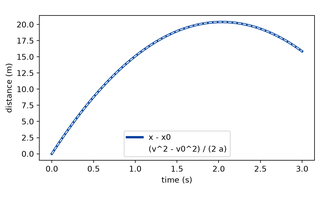
Lean exercises on your machine
Three theorems of constant acceleration and of an impulse between two particles, given as Lean 4 stubs to complete locally, with hints, and with the solutions that CI compiles, read from the repository.
Intermediate, level 2 of 3
Details of Lean exercises on your machine
Course
Classical mechanics
Methods
Formal proofs
Level
Intermediate, level 2 of 3
What you build
Three theorems of constant acceleration and of an impulse between two particles, given as Lean 4 stubs to complete locally, with hints, and with the solutions that CI compiles, read from the repository.
What you’ll learn
- Complete a Lean 4 stub on your own machine and check it with the pinned toolchain
- Prove an identity of constant acceleration and a momentum balance by substitution and algebra
- Say why the site shows a stub as not verified and a solution as checked
Prerequisites
Proving what the simulation showed. Also assumed: Logic: reading a statement that says if these hypotheses hold, then this conclusion holds; Algebra: expanding and factorising polynomials in several variables.
Related
none
On your machine
Check this proof
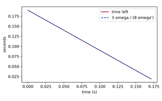
The chirp law, proved
The shrinking orbit, the rate of the frequency, the chirp mass, and the time to coalescence of the gravitational-wave strain lab, stated and proved in Lean 4 as exact consequences of Kepler's third law and an assumed energy loss, and what that says about the model and nothing about the measurement.
Advanced, level 3 of 3
Details of The chirp law, proved
Course
Classical mechanics
Methods
Formal proofs
Level
Advanced, level 3 of 3
What you build
The shrinking orbit, the rate of the frequency, the chirp mass, and the time to coalescence of the gravitational-wave strain lab, stated and proved in Lean 4 as exact consequences of Kepler's third law and an assumed energy loss, and what that says about the model and nothing about the measurement.
What you’ll learn
- State the shrink rate of a circular orbit and the chirp rate as theorems in Lean 4, with the quadrupole power as a hypothesis
- Read the proof that a frequency and its rate fix the chirp mass, and the proof that the time to coalescence counts down at the rate one
- Say that the theorems are about the model of the lab, and that they prove nothing about the measured strain or the masses of the black holes
Prerequisites
Gravitational-wave strain lab, Proving what the simulation showed. Also assumed: Calculus: the chain rule and the derivative of a power and of a quotient.
Related
none
On your machine
Check this proof

Dependency map of Classical mechanics

Kinematics as a program has the related lesson Proving what the simulation showed (recommended, not required).
Newton’s laws as a first-order system requires Kinematics as a program.
Projectile motion with quadratic drag requires Newton’s laws as a first-order system.
Projectile motion with quadratic drag has the related lesson An agent runs an experiment (recommended, not required).
The harmonic oscillator requires Newton’s laws as a first-order system.
The harmonic oscillator has the related lesson Proving what the simulation showed (recommended, not required).
Numerical integrators requires The harmonic oscillator.
Numerical integrators has the related lesson What symplectic Euler conserves (recommended, not required).
Energy conservation requires Numerical integrators.
Momentum and collisions requires Energy conservation.
Momentum and collisions has the related lesson Momentum in a collision, proved (recommended, not required).
The Kepler orbit requires Energy conservation.
The Kepler orbit requires Momentum and collisions.
The Kepler orbit has the related lesson Gravitational-wave strain lab (recommended, not required).
Double pendulum and chaos requires Numerical integrators.
Double pendulum and chaos requires Energy conservation.
Double pendulum and chaos has the related lesson Lagrangian mechanics (recommended, not required).
Lagrangian mechanics requires Energy conservation.
Lagrangian mechanics requires Double pendulum and chaos.
Lagrangian mechanics has the related lesson Hamiltonian mechanics (recommended, not required).
Hamiltonian mechanics requires Numerical integrators.
Hamiltonian mechanics requires Lagrangian mechanics.
Hamiltonian mechanics requires What symplectic Euler conserves.
Resonance and driven oscillators requires Projectile motion with quadratic drag.
Resonance and driven oscillators requires The harmonic oscillator.
Resonance and driven oscillators requires Numerical integrators.
Gravitational-wave strain lab requires The Kepler orbit.
Gravitational-wave strain lab has the related lesson The chirp law, proved (recommended, not required).
An agent runs an experiment requires Projectile motion with quadratic drag.
Verifying scientific code requires Numerical integrators.
Verifying scientific code requires Energy conservation.
A counterexample hunter requires Numerical integrators.
A counterexample hunter requires An agent runs an experiment.
A counterexample hunter has the related lesson Verifying scientific code (recommended, not required).
Three reviewers for one piece of code requires An agent runs an experiment.
Three reviewers for one piece of code requires Verifying scientific code.
Discovering a force law with controlled probes requires An agent runs an experiment.
Discovering a force law with controlled probes requires Inverse physics: parameters from observations.
Full, partial, and no prior knowledge under one protocol requires The harmonic oscillator.
Full, partial, and no prior knowledge under one protocol requires Discovering a force law with controlled probes.
Unlearning a familiar law: a modified force requires The Kepler orbit.
Unlearning a familiar law: a modified force requires Discovering a force law with controlled probes.
Inverse physics: parameters from observations requires The harmonic oscillator.
Inverse physics: parameters from observations requires Gravitational-wave strain lab.
An agent that designs the measurements requires A counterexample hunter.
An agent that designs the measurements requires Inverse physics: parameters from observations.
Automated analysis pipelines requires Projectile motion with quadratic drag.
Proving what the simulation showed requires Kinematics as a program.
Proving what the simulation showed requires The harmonic oscillator.
Momentum in a collision, proved requires Momentum and collisions.
Momentum in a collision, proved requires Proving what the simulation showed.
What symplectic Euler conserves requires Numerical integrators.
What symplectic Euler conserves requires Proving what the simulation showed.
Lean exercises on your machine requires Proving what the simulation showed.
The chirp law, proved requires Gravitational-wave strain lab.
The chirp law, proved requires Proving what the simulation showed.

Thermodynamics and statistical physics

Preview, simulated: Histogram of disc speeds in metres per second. The bars rise from zero at zero speed to a single peak and fall off in a long tail, and a dashed curve of the Maxwell distribution follows the tops of the bars closely.

Heat, entropy, and equilibrium built from the motion of many particles: random walks, kinetic theory, the Ising model, and molecular dynamics.

4 published lessons, 8 planned.

Start with Particles in a box

Lessons of Thermodynamics and statistical physics (4 published)

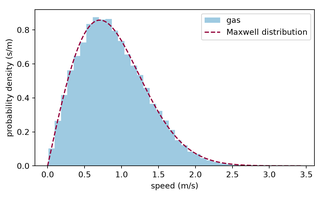
Particles in a box
A gas of colliding discs built from one local rule, and the pressure and the distribution of speeds that emerge from it, checked against kinetic theory within a stated statistical tolerance.
Intermediate, level 2 of 3
- Simulation
Details of Particles in a box
Course
Thermodynamics and statistical physics
Slot
T0, Gas from simple agents
Methods
Simulation, Agent-based modelling
Level
Intermediate, level 2 of 3
What you build
A gas of colliding discs built from one local rule, and the pressure and the distribution of speeds that emerge from it, checked against kinetic theory within a stated statistical tolerance.
What you’ll learn
- Build a gas of colliding discs from one local rule
- Measure the pressure and the distribution of speeds that emerge
- Check them against kinetic theory within a stated statistical tolerance
Prerequisites
Momentum and collisions. Also assumed: Statistics: the mean, the standard deviation, and the standard error of a mean; Probability: the Gaussian distribution and the t distribution.
Related
none
On your machine
Run this experiment
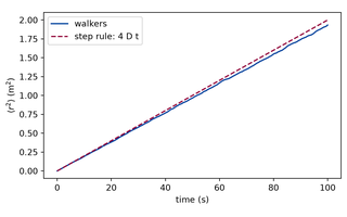
Random walks and diffusion
A walker that takes one random step at a time, the diffusion law that many of them obey, and the diffusion coefficient measured from the walk and checked against the value the step rule predicts.
Introductory, level 1 of 3
- Simulation
Details of Random walks and diffusion
Course
Thermodynamics and statistical physics
Slot
T1, Random walks and diffusion
Methods
Simulation
Level
Introductory, level 1 of 3
What you build
A walker that takes one random step at a time, the diffusion law that many of them obey, and the diffusion coefficient measured from the walk and checked against the value the step rule predicts.
What you’ll learn
- Build a random walk from one rule for a single step
- Measure the mean squared displacement of many walkers and the diffusion coefficient it gives
- Check the measured coefficient and the spread of the walkers against what the step rule predicts
Prerequisites
Kinematics as a program. Also assumed: Statistics: the mean, the variance, and the standard error of a mean; Probability: independent random variables, and the Gaussian distribution.
Related
none
On your machine
Run this experiment
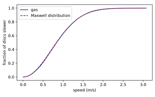
Kinetic theory of gases
Why a gas of colliding particles settles into the Maxwell distribution of speeds, and a check of the simulated gas of the first lesson against the analytic distribution at the temperature the simulation reached.
Intermediate, level 2 of 3
- Simulation
Details of Kinetic theory of gases
Course
Thermodynamics and statistical physics
Slot
T2, Kinetic theory of gases
Methods
Simulation
Level
Intermediate, level 2 of 3
What you build
Why a gas of colliding particles settles into the Maxwell distribution of speeds, and a check of the simulated gas of the first lesson against the analytic distribution at the temperature the simulation reached.
What you’ll learn
- Derive the Maxwell distribution of speeds from the independence and the isotropy of the velocity components
- Define the temperature of a gas from its mean kinetic energy
- Check the speeds of a simulated gas against the analytic distribution at its own temperature, within a stated tolerance
Prerequisites
Particles in a box. Also assumed: Probability: the Gaussian distribution, the distribution function of a random variable, and its quantiles; Statistics: the mean, the standard deviation, and the standard error of a mean; Calculus: integrating a Gaussian, and changing to polar coordinates.
Related
Random walks and diffusion
On your machine
Run this experiment
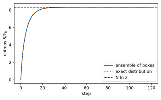
Entropy from ensembles
Entropy as the logarithm of a count of microstates, grown from an ensemble of boxes of particles, checked against a case with a closed form, and the limits of what an estimate of an entropy can tell.
Intermediate, level 2 of 3
- Simulation
Details of Entropy from ensembles
Course
Thermodynamics and statistical physics
Slot
T3, Entropy and thermodynamic equilibrium
Methods
Simulation
Level
Intermediate, level 2 of 3
What you build
Entropy as the logarithm of a count of microstates, grown from an ensemble of boxes of particles, checked against a case with a closed form, and the limits of what an estimate of an entropy can tell.
What you’ll learn
- Count the microstates of a macrostate and write the entropy as the logarithm of the count
- Evolve an ensemble of boxes and estimate its entropy from the observed frequencies
- Check the entropy of the ensemble against its value at equilibrium, and say what an estimate from a finite ensemble can and cannot show
Prerequisites
Random walks and diffusion. Also assumed: Probability: probabilities of independent events, and the binomial distribution; Logarithms: the natural logarithm of a product, and of a factorial for large numbers; Statistics: the mean, the standard deviation, and the standard error of a mean.
Related
Kinetic theory of gases
On your machine
Run this experiment
T4 Ising model and phase transitions (planned, not published)
T5 Molecular dynamics (planned, not published)
T6 Heat conduction and diffusion (planned, not published)
T9 Heat engines and thermodynamic cycles (planned, not published)
T10 From finite differences to finite elements and meshes (planned, not published)
T11 Applied capstone: thermal engineering of an AI accelerator, applied capstone (planned, not published)
T7 Experimental: heat transfer measurements, measured-data lab (planned, not published)
T8 Experimental: Brownian motion tracking, measured-data lab (planned, not published)

Dependency map of Thermodynamics and statistical physics

Waves and optics

Preview, simulated: Five stacked curves of displacement against position along a string from zero to one metre. The top curve is a single bump near the left. Below it the bump has split in two halves that move apart, then the right half reaches the right end and a half of opposite sign, pointing down, appears to come back from it.

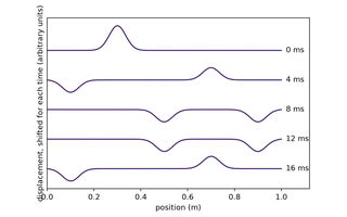
Waves and what they do: interference, refraction, polarisation, diffraction, and the inverse problem of imaging.

3 published lessons, 6 planned.

Start with The wave equation

Lessons of Waves and optics (3 published)

The wave equation
A pulse on a string, solved by finite differences: how the scheme is derived, how its error falls as the grid is refined, and where the Courant number sets a limit that no refinement of the grid can move.
Intermediate, level 2 of 3
- Simulation
Details of The wave equation
Course
Waves and optics
Slot
W1, The wave equation
Methods
Simulation
Level
Intermediate, level 2 of 3
What you build
A pulse on a string, solved by finite differences: how the scheme is derived, how its error falls as the grid is refined, and where the Courant number sets a limit that no refinement of the grid can move.
What you’ll learn
- Derive the leapfrog scheme for the wave equation from centred differences
- Measure the order of convergence of the scheme against an exact solution
- Show that a Courant number above one makes the scheme grow without bound, at the rate the theory predicts
Prerequisites
The harmonic oscillator, Numerical integrators. Also assumed: Calculus: partial derivatives, and the Taylor expansion of a function to second order; Numerical methods: the order of a method and how it is measured from the error at two step sizes.
Related
none
On your machine
Run this experiment
Interference and resonance
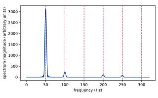
Waves add: pulses pass through each other, a plucked string sounds at its mode frequencies, a push at one of them builds up without limit, a grid disperses what the equation does not, and two sources make a pattern.
Intermediate, level 2 of 3
- Simulation
Details of Interference and resonance
Course
Waves and optics
Slot
W2, Interference and resonance
Methods
Simulation
Level
Intermediate, level 2 of 3
What you build
Waves add: pulses pass through each other, a plucked string sounds at its mode frequencies, a push at one of them builds up without limit, a grid disperses what the equation does not, and two sources make a pattern.
What you’ll learn
- Use the linearity of the wave equation to build standing waves and modes from travelling ones
- Check the frequencies of a simulated string against the analytic mode frequencies
- Show a resonance, and measure the dispersion that a grid adds to a wave
- Predict the pattern of two coherent sources and check it by adding their waves
Prerequisites
The wave equation. Also assumed: Trigonometry: the sum of two sines, and the identity for the product of a sine and a cosine; Complex numbers: the form exp(i x) of a wave and the modulus of a sum.
Related
none
On your machine
Run this experiment
W3 Refraction and Snell's law (planned, not published)
W4 Polarisation and Malus's law (planned, not published)
W5 Diffraction and imaging (planned, not published)
W6 Inverse optics (planned, not published)
Sound, resonance, and the Doppler effect
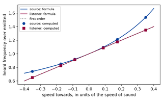
Sound as a pressure wave computed on a grid: the resonances of open and closed pipes, a sweep through them, and the shift in pitch of a moving source or a moving listener, each checked against its formula.
Intermediate, level 2 of 3
- Simulation
Details of Sound, resonance, and the Doppler effect
Course
Waves and optics
Slot
W9, Sound waves, resonance, and the Doppler effect
Methods
Simulation
Level
Intermediate, level 2 of 3
What you build
Sound as a pressure wave computed on a grid: the resonances of open and closed pipes, a sweep through them, and the shift in pitch of a moving source or a moving listener, each checked against its formula.
What you’ll learn
- Compute the resonances of an open and of a closed pipe from the wave equation and check them against the analytic frequencies
- Find the resonances of a pipe by sweeping the frequency of a driving force
- Compute the pitch that a listener hears from a moving source and for a moving listener, and check it against both Doppler formulas
Prerequisites
The wave equation, Interference and resonance. Also assumed: Calculus: partial derivatives, and the linearisation of a function about a point.
Related
none
On your machine
Run this experiment
W7 Experimental: real optical diffraction images, measured-data lab (planned, not published)
W8 Experimental: wave flume measurements, measured-data lab (planned, not published)

Dependency map of Waves and optics

Electromagnetism

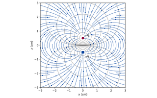
Preview, simulated: A square plot of the plane through two charges, a positive one above and a negative one below the centre. Blue curved lines run from the upper charge out and around to the lower charge, dense near the charges and spreading out far away. Thin grey closed curves, the equipotentials, surround each charge and cross the field lines at right angles. The pattern is symmetric about the line through both charges.

Electric and magnetic fields from Coulomb's law to Maxwell's equations, solved on a grid and checked against measurements.

3 published lessons, 6 planned.

Start with Electric fields, superposition, and the potential

Lessons of Electromagnetism (3 published)

Electric fields, superposition, and the potential
The electric field of point charges computed by adding Coulomb's law charge by charge, checked against minus the gradient of the potential, against the closed form of a dipole far away, and against Gauss's law on a sphere.
Introductory, level 1 of 3
- Simulation
Details of Electric fields, superposition, and the potential
Course
Electromagnetism
Slot
EM1, Coulomb's law and electric fields
Methods
Simulation
Level
Introductory, level 1 of 3
What you build
The electric field of point charges computed by adding Coulomb's law charge by charge, checked against minus the gradient of the potential, against the closed form of a dipole far away, and against Gauss's law on a sphere.
What you’ll learn
- Compute the electric field of a set of point charges as a vector field, by superposition of Coulomb's law
- Obtain the field from the potential by a numerical gradient and measure the order of its error
- Check the field of a pair of charges against the closed form of a dipole, and say how fast the two agree with distance
- Check Gauss's law by computing the flux through a sphere around and beside the charges
Prerequisites
Newton’s laws as a first-order system. Also assumed: Vectors: components, the dot product, and the gradient of a function of the position; Calculus: partial derivatives, and integrals over a surface.
Related
none
On your machine
Run this experiment
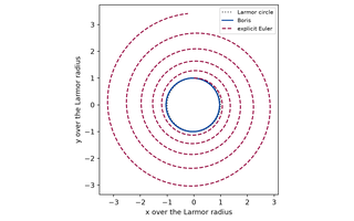
Charged particles in electric and magnetic fields
The Lorentz force integrated with the Boris pusher: a proton circles in a magnetic field at the cyclotron frequency and the Larmor radius, keeps its energy where explicit Euler does not, and drifts across crossed fields at E over B, each checked against its formula.
Intermediate, level 2 of 3
- Simulation
Details of Charged particles in electric and magnetic fields
Course
Electromagnetism
Slot
EM2, Lorentz force and charged particles
Methods
Simulation
Level
Intermediate, level 2 of 3
What you build
The Lorentz force integrated with the Boris pusher: a proton circles in a magnetic field at the cyclotron frequency and the Larmor radius, keeps its energy where explicit Euler does not, and drifts across crossed fields at E over B, each checked against its formula.
What you’ll learn
- Integrate the motion of a charged particle under the Lorentz force with the Boris pusher
- Measure the cyclotron frequency and the Larmor radius of a simulated orbit and check them against qB/m and mv/(qB)
- Predict the error of the Boris pusher from its own closed form and measure its order
- Explain why explicit Euler gains energy in a magnetic field, and compute the drift of a particle in crossed fields
Prerequisites
Electric fields, superposition, and the potential, Numerical integrators. Also assumed: Vectors: the cross product in three dimensions; Trigonometry: the tangent of a half angle.
Related
none
On your machine
Run this experiment
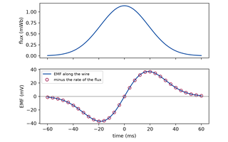
Induction: magnetic flux and the electromotive force
The voltage induced around a loop computed as the work per charge along the wire, and the magnetic flux through it computed as a surface integral, apart: for a loop moving through a non-uniform field, a turning coil, and a loop at rest beside a changing field, the voltage is minus the rate of change of the flux.
Intermediate, level 2 of 3
- Simulation
Details of Induction: magnetic flux and the electromotive force
Course
Electromagnetism
Slot
EM3, Faraday's law and induction
Methods
Simulation
Level
Intermediate, level 2 of 3
What you build
The voltage induced around a loop computed as the work per charge along the wire, and the magnetic flux through it computed as a surface integral, apart: for a loop moving through a non-uniform field, a turning coil, and a loop at rest beside a changing field, the voltage is minus the rate of change of the flux.
What you’ll learn
- Compute the magnetic flux through a loop as a surface integral and its rate of change by a central difference
- Compute the electromotive force around a loop as the line integral of the force per charge on the charges of the wire
- Check Faraday's law for a moving loop, a turning coil, and a loop at rest in a changing field
- Explain why a loop can have an induced voltage where the magnetic field on the wire is nearly zero, and none where the electric field is not
Prerequisites
Electric fields, superposition, and the potential, Charged particles in electric and magnetic fields. Also assumed: Vectors: the cross product in three dimensions; Calculus: line integrals and integrals over a surface.
Related
none
On your machine
Run this experiment
EM4 Maxwell's equations and FDTD (planned, not published)
EM5 RLC circuits and resonance (planned, not published)
EM6 Waveguides and electromagnetic resonances (planned, not published)
EM7 Experimental: microwave S-parameters, measured-data lab (planned, not published)
EM8 Experimental: real RLC circuit measurements, measured-data lab (planned, not published)
EM9 Applied capstone: adaptive phased-array beam steering, applied capstone (planned, not published)

Dependency map of Electromagnetism

Method paths

A method path is a second way through the same lessons: the lessons that fill the slots of one path of the reference curriculum, in the order of the path. It is not a course and has no pages of its own; each entry links to the lesson in its course, and a lesson belongs to at most one path.

Physics reasoning and scientific agents

4 published lessons, 5 planned

An agent runs an experiment Classical mechanics, intermediate, level 2 of 3
AI1 Agent-assisted physics simulation development (planned, not published)
Verifying scientific code Classical mechanics, advanced, level 3 of 3
A counterexample hunter Classical mechanics, advanced, level 3 of 3
Three reviewers for one piece of code Classical mechanics, advanced, level 3 of 3
AI5 Agent-assisted real experimental physics (planned, not published)
AI6 Multimodal physics reasoning (planned, not published)
AI7 Interpretable physics explanations and constraints (planned, not published)
AI8 Physical reasoning from video (planned, not published)

Scientific law discovery

5 published lessons, 8 planned

Discovering a force law with controlled probes Classical mechanics, intermediate, level 2 of 3
Full, partial, and no prior knowledge under one protocol Classical mechanics, advanced, level 3 of 3
Unlearning a familiar law: a modified force Classical mechanics, advanced, level 3 of 3
D4 Discovering gravity from experiments (planned, not published)
D5 Unknown physical worlds (planned, not published)
Inverse physics: parameters from observations Classical mechanics, advanced, level 3 of 3
D7 Symbolic regression for physical laws (planned, not published)
D8 Discovering differential equations (planned, not published)
An agent that designs the measurements Classical mechanics, advanced, level 3 of 3
D10 Scientific discovery under measurement noise (planned, not published)
D11 Hidden forces and unobserved variables (planned, not published)
D12 Generalisation to unseen physical systems (planned, not published)
D13 Discovering conservation laws and physical invariants (planned, not published)

Physics agent benchmarking

0 published lessons, 5 planned

EV1 Physics reasoning benchmarks (planned, not published)
EV2 Interactive discovery benchmarks (planned, not published)
EV3 Agent versus non-agent baselines (planned, not published)
EV4 Robustness, cost, and sample efficiency (planned, not published)
EV5 Scientific failure analysis (planned, not published)

Autonomous scientific research

1 published lesson, 5 planned

Automated analysis pipelines Classical mechanics, intermediate, level 2 of 3
R2 Scientific evidence maps (planned, not published)
R3 Scientific literature and reproducible evidence (planned, not published)
R4 Reproducing a physics paper with multiple agents (planned, not published)
R5 Agent-driven materials discovery (planned, not published)
R6 Autonomous physics research challenge (planned, not published)

Methods

A method is a way of working that cuts across courses. Each list links the lessons that use the method, in the order of the learning path.

Simulation

Lessons that build a model as a program and check it against theory.

Kinematics as a program Classical mechanics, introductory, level 1 of 3
Newton’s laws as a first-order system Classical mechanics, intermediate, level 2 of 3
Projectile motion with quadratic drag Classical mechanics, intermediate, level 2 of 3
The harmonic oscillator Classical mechanics, intermediate, level 2 of 3
Numerical integrators Classical mechanics, intermediate, level 2 of 3
Energy conservation Classical mechanics, intermediate, level 2 of 3
Momentum and collisions Classical mechanics, intermediate, level 2 of 3
The Kepler orbit Classical mechanics, advanced, level 3 of 3
Verifying scientific code Classical mechanics, advanced, level 3 of 3
Automated analysis pipelines Classical mechanics, intermediate, level 2 of 3
Gravitational-wave strain lab Classical mechanics, advanced, level 3 of 3
Inverse physics: parameters from observations Classical mechanics, advanced, level 3 of 3
Double pendulum and chaos Classical mechanics, advanced, level 3 of 3
Lagrangian mechanics Classical mechanics, advanced, level 3 of 3
Hamiltonian mechanics Classical mechanics, advanced, level 3 of 3
Resonance and driven oscillators Classical mechanics, intermediate, level 2 of 3
Random walks and diffusion Thermodynamics and statistical physics, introductory, level 1 of 3
Kinetic theory of gases Thermodynamics and statistical physics, intermediate, level 2 of 3
Entropy from ensembles Thermodynamics and statistical physics, intermediate, level 2 of 3
The wave equation Waves and optics, intermediate, level 2 of 3
Interference and resonance Waves and optics, intermediate, level 2 of 3
Sound, resonance, and the Doppler effect Waves and optics, intermediate, level 2 of 3
Electric fields, superposition, and the potential Electromagnetism, introductory, level 1 of 3
Charged particles in electric and magnetic fields Electromagnetism, intermediate, level 2 of 3
Induction: magnetic flux and the electromotive force Electromagnetism, intermediate, level 2 of 3
An agent runs an experiment Classical mechanics, intermediate, level 2 of 3
A counterexample hunter Classical mechanics, advanced, level 3 of 3
Three reviewers for one piece of code Classical mechanics, advanced, level 3 of 3
An agent that designs the measurements Classical mechanics, advanced, level 3 of 3
Discovering a force law with controlled probes Classical mechanics, intermediate, level 2 of 3
Full, partial, and no prior knowledge under one protocol Classical mechanics, advanced, level 3 of 3
Unlearning a familiar law: a modified force Classical mechanics, advanced, level 3 of 3
Particles in a box Thermodynamics and statistical physics, intermediate, level 2 of 3

LLM agents

Lessons in which a language model proposes and runs experiments with the simulation code, on your own machine with your own API key.

An agent runs an experiment Classical mechanics, intermediate, level 2 of 3
A counterexample hunter Classical mechanics, advanced, level 3 of 3
Three reviewers for one piece of code Classical mechanics, advanced, level 3 of 3
An agent that designs the measurements Classical mechanics, advanced, level 3 of 3
Discovering a force law with controlled probes Classical mechanics, intermediate, level 2 of 3
Full, partial, and no prior knowledge under one protocol Classical mechanics, advanced, level 3 of 3
Unlearning a familiar law: a modified force Classical mechanics, advanced, level 3 of 3

Agent-based modelling

Lessons with many simple agents, local rules, and the collective behaviour that emerges from them.

Particles in a box Thermodynamics and statistical physics, intermediate, level 2 of 3

Formal proofs

Lessons that state results as theorems in Lean 4 with Mathlib and check them by machine.

Proving what the simulation showed Classical mechanics, intermediate, level 2 of 3
Momentum in a collision, proved Classical mechanics, intermediate, level 2 of 3
What symplectic Euler conserves Classical mechanics, advanced, level 3 of 3
Lean exercises on your machine Classical mechanics, intermediate, level 2 of 3
The chirp law, proved Classical mechanics, advanced, level 3 of 3

Measured data

Lessons that compare a model with measurements.

Automated analysis pipelines Classical mechanics, intermediate, level 2 of 3
Gravitational-wave strain lab Classical mechanics, advanced, level 3 of 3
Inverse physics: parameters from observations Classical mechanics, advanced, level 3 of 3

Difficulty

Every lesson states one of 3 levels.

1, introductory: Builds one idea from the outside prerequisites alone and shows every step.
2, intermediate: Builds on earlier lessons and combines their ideas. The exercises need more than the worked examples show.
3, advanced: Longer derivations, experiments, or proofs, with exercises that leave the route to you.

Order

Three orders are in use, and they are not the same.

Previous and next on a lesson page follow the one linear order of the site: the courses and then the method strands one after the other (Classical mechanics, then Thermodynamics and statistical physics, then Waves and optics, then Electromagnetism, then Physics and AI: LLM agents, then Agent-based modelling, then Formal proofs), and within a strand the lessons by their number. Following next from the last lesson of one strand leads to the first lesson of the following strand, which may belong to another course.

The course order and the path order are the teaching order of the reference curriculum: the lessons of a course or a path in the order of their slots in the curriculum file, which may differ from the order of the labels, and the lessons without a slot after them in the linear order.

The prerequisites of a lesson are the lessons it builds on, and are the only statement of what you need first. A prerequisite may live in a later strand, so previous and next may lead to a lesson before one it builds on: the header of every lesson links its prerequisites, and the dependency map below gives the order of ideas.

Your progress

This site can remember which lessons you have completed and how you answered the self-checks. It keeps that in your browser and nowhere else, in local storage under the key physics-by-construction:learner-state: for each lesson, whether you marked it completed, whether you finished its self-check, and how often you checked an answer, and which suggestions you ignored. No account is needed. Nothing is sent to a server, no cookie is set, and nothing is shared with other sites or other devices. Clearing the data of this site in your browser removes it too, and so does the button below.

Without scripts nothing is stored, and the self-checks work as exercises with a solution you can open.

With scripts, this place shows which lessons you have completed and a button that clears them.

With scripts, this place suggests what to do next, with the reason, from the progress saved in your browser. Without them, follow the learning path.

Prerequisite graph

The graph shows the same prerequisites as the lessons above, as a picture. Each box is a lesson and links to it. A lesson stands one column to the right of its furthest prerequisite, and the lessons of a course share a band. It is optional: every prerequisite is also named in the details of its lesson. On a narrow screen the graph scrolls sideways inside its box.

View dependency map

Requires: a solid line with a filled arrowhead, from a prerequisite to the lesson that needs it.
Related: a dashed line with an open arrowhead, from a lesson to a lesson it recommends as an extension; not required.

Kinematics as a program has the related lesson Proving what the simulation showed (recommended, not required).
Newton’s laws as a first-order system requires Kinematics as a program.
Projectile motion with quadratic drag requires Newton’s laws as a first-order system.
Projectile motion with quadratic drag has the related lesson An agent runs an experiment (recommended, not required).
The harmonic oscillator requires Newton’s laws as a first-order system.
The harmonic oscillator has the related lesson Proving what the simulation showed (recommended, not required).
Numerical integrators requires The harmonic oscillator.
Numerical integrators has the related lesson What symplectic Euler conserves (recommended, not required).
Energy conservation requires Numerical integrators.
Momentum and collisions requires Energy conservation.
Momentum and collisions has the related lesson Particles in a box (recommended, not required).
Momentum and collisions has the related lesson Momentum in a collision, proved (recommended, not required).
The Kepler orbit requires Energy conservation.
The Kepler orbit requires Momentum and collisions.
The Kepler orbit has the related lesson Gravitational-wave strain lab (recommended, not required).
Verifying scientific code requires Numerical integrators.
Verifying scientific code requires Energy conservation.
Automated analysis pipelines requires Projectile motion with quadratic drag.
Gravitational-wave strain lab requires The Kepler orbit.
Gravitational-wave strain lab has the related lesson The chirp law, proved (recommended, not required).
Inverse physics: parameters from observations requires The harmonic oscillator.
Inverse physics: parameters from observations requires Gravitational-wave strain lab.
Double pendulum and chaos requires Numerical integrators.
Double pendulum and chaos requires Energy conservation.
Double pendulum and chaos has the related lesson Lagrangian mechanics (recommended, not required).
Lagrangian mechanics requires Energy conservation.
Lagrangian mechanics requires Double pendulum and chaos.
Lagrangian mechanics has the related lesson Hamiltonian mechanics (recommended, not required).
Hamiltonian mechanics requires Numerical integrators.
Hamiltonian mechanics requires Lagrangian mechanics.
Hamiltonian mechanics requires What symplectic Euler conserves.
Resonance and driven oscillators requires Projectile motion with quadratic drag.
Resonance and driven oscillators requires The harmonic oscillator.
Resonance and driven oscillators requires Numerical integrators.
Random walks and diffusion requires Kinematics as a program.
Kinetic theory of gases requires Particles in a box.
Kinetic theory of gases has the related lesson Random walks and diffusion (recommended, not required).
Entropy from ensembles requires Random walks and diffusion.
Entropy from ensembles has the related lesson Kinetic theory of gases (recommended, not required).
The wave equation requires The harmonic oscillator.
The wave equation requires Numerical integrators.
Interference and resonance requires The wave equation.
Sound, resonance, and the Doppler effect requires The wave equation.
Sound, resonance, and the Doppler effect requires Interference and resonance.
Electric fields, superposition, and the potential requires Newton’s laws as a first-order system.
Charged particles in electric and magnetic fields requires Numerical integrators.
Charged particles in electric and magnetic fields requires Electric fields, superposition, and the potential.
Induction: magnetic flux and the electromotive force requires Electric fields, superposition, and the potential.
Induction: magnetic flux and the electromotive force requires Charged particles in electric and magnetic fields.
An agent runs an experiment requires Projectile motion with quadratic drag.
A counterexample hunter requires Numerical integrators.
A counterexample hunter requires An agent runs an experiment.
A counterexample hunter has the related lesson Verifying scientific code (recommended, not required).
Three reviewers for one piece of code requires Verifying scientific code.
Three reviewers for one piece of code requires An agent runs an experiment.
An agent that designs the measurements requires Inverse physics: parameters from observations.
An agent that designs the measurements requires A counterexample hunter.
Discovering a force law with controlled probes requires Inverse physics: parameters from observations.
Discovering a force law with controlled probes requires An agent runs an experiment.
Full, partial, and no prior knowledge under one protocol requires The harmonic oscillator.
Full, partial, and no prior knowledge under one protocol requires Discovering a force law with controlled probes.
Unlearning a familiar law: a modified force requires The Kepler orbit.
Unlearning a familiar law: a modified force requires Discovering a force law with controlled probes.
Particles in a box requires Momentum and collisions.
Proving what the simulation showed requires Kinematics as a program.
Proving what the simulation showed requires The harmonic oscillator.
Momentum in a collision, proved requires Momentum and collisions.
Momentum in a collision, proved requires Proving what the simulation showed.
What symplectic Euler conserves requires Numerical integrators.
What symplectic Euler conserves requires Proving what the simulation showed.
Lean exercises on your machine requires Proving what the simulation showed.
The chirp law, proved requires Gravitational-wave strain lab.
The chirp law, proved requires Proving what the simulation showed.