Particles in a box

A gas of colliding discs built from one local rule, and the pressure and the distribution of speeds that emerge from it, checked against kinetic theory within a stated statistical tolerance.

Course

Thermodynamics and statistical physics, lesson 1 of 4

Slot

T0, Gas from simple agents

Methods

Simulation, Agent-based modelling

Difficulty

Intermediate, level 2 of 3

What you’ll learn

Build a gas of colliding discs from one local rule
Measure the pressure and the distribution of speeds that emerge
Check them against kinetic theory within a stated statistical tolerance

Prerequisites

Momentum and collisions.

Before you begin

Statistics: the mean, the standard deviation, and the standard error of a mean
Probability: the Gaussian distribution and the t distribution

Related

none

Previous

Unlearning a familiar law: a modified force

Next

Proving what the simulation showed

With scripts, this page keeps a record in your browser of whether you completed the lesson. Nothing is stored without them.

With scripts, this place suggests what to do next, with the reason, from the progress saved in your browser. Without them, follow the learning path.

Why does a gas push on the walls of its container with a steady pressure, and why do the speeds of its molecules follow one particular curve, when each molecule only ever meets a wall or a neighbour? Neither the pressure nor the curve belongs to any molecule. They belong to the many. A model that wants to reproduce them has to produce them without being told.

An agent-based model has no equation for the whole system. It has many agents, each following a simple rule that refers only to what is near it, and it runs them. This lesson builds the smallest such model of physics: a gas of identical discs in a box. A disc moves in a straight line, bounces off a wall, and collides elastically with a disc it touches, the collision of the momentum and collisions lesson. No rule mentions pressure, temperature, or a distribution of speeds.

The lesson then measures these from the whole. The pressure on the walls is the impulse the walls gave, per second and per length. The distribution of speeds is read off the discs. Both can be predicted by kinetic theory, so the model has something to be checked against: collisions that start from discs of one speed should produce the Maxwell distribution, and the walls should feel the pressure of the gas law. The checks are statistical, because the model is random; the lesson states the tolerance and says what it means. They are numerical checks of a model against a theory. No real gas is measured here.

Assumptions

Two dimensions, identical hard discs. Every disc has the same radius and mass, and discs are smooth, so a collision exchanges momentum along the line of centres only and nothing spins. In three dimensions the speeds follow the three-dimensional Maxwell distribution and the numbers below change; the method does not.
Elastic collisions and perfectly reflecting walls. Kinetic energy is conserved by every collision and every bounce. A wall at rest only reverses the normal velocity, so it gives momentum to the gas but no energy. With dissipation the gas would cool, and there would be no temperature to compare.
The gas is dilute. The area of the discs is a small fraction $\varphi$ of the area their centres can reach. Collisions then involve two discs at a time, and the first correction to the ideal gas law, the area the discs exclude, is enough. This is the first term of a series in $\varphi$ ; the test of the code compares the pressure with this one term at the packing fraction used, within a stated allowance for what the term leaves out and the statistical error. A dense gas needs more of the series, and a collision of three discs at once is outside the model.
The time step resolves a collision. The program moves all discs by $\Delta t$ , then collides the pairs that overlap and approach each other, one pair after the other. A disc therefore overlaps another by up to the distance it moves in one step, and a collision is placed at the end of the step, not at the moment of contact. The step must be small against the diameter, or two discs pass through each other. The first worked example prints the distance a disc moves in a step as a fraction of the diameter. A collision placed late also lowers the pressure a little, and the comparison with theory allows for it.
The gas has relaxed before it is measured. The start is not a Maxwell distribution. Every disc is first given the same speed in a random direction; the mean velocity is then removed, so that the gas has no bulk motion, and the velocities are rescaled to the stated kinetic energy. Removing the mean velocity changes each speed a little, so the discs start in a narrow band of speeds around the stated root-mean-square speed. The measurement begins after the collisions have had time to change that, and the lesson shows it happening.
The runs are independent, the discs in a run are not. The discs of one run share energy through their collisions, and one disc at successive times is correlated with itself. The standard error of a quantity is therefore computed from the spread between independent runs started from different seeds, never from the number of discs or snapshots.
Randomness is seeded. A random number generator created from a seed makes the start of a run, so a run is a function of its inputs and the page is the same at every build on one machine. The collisions amplify every difference, so on another machine, whose floating-point libraries round differently, a run of the same seed soon follows another path: it is, in effect, another sample of the same gas. The digits can then differ, and the check is built so that its verdict does not (see “What the tolerance means”).

Explanation

From a local rule to a whole

The state of the model is a position and a velocity for each disc. One step does three things in order:

every disc moves, $\mathbf x \leftarrow \mathbf x + \mathbf v\,\Delta t$ ;
a disc that crossed a wall is put back inside and the component of its velocity normal to the wall is reversed;
every pair of discs that overlap and are still approaching collides elastically: the relative velocity along the line of centres reverses, the rest is unchanged (hard_sphere_collision of the earlier lesson).

The second and third steps are the only places where discs affect anything, and each involves a disc and its immediate neighbour or wall. The pressure and the distribution of speeds below are properties of the many, not of any rule. That is what is meant by emergent here: the rules are written once for one agent, and the quantity is found only by running all of them.

Pressure

A disc of mass $m$ that bounces off a wall with normal speed $v_n$ gives the wall the impulse $2 m v_n$ . Add the impulses over a time $T$ and divide by the time and by the length of the wall, $4 L$ for a square of side $L$ , and the result is a force per length, the pressure of a two-dimensional gas.

Kinetic theory predicts the value for point particles. In a short time $\Delta t$ the discs that hit a wall of length $\ell$ are those that move towards it and are within $v_n\,\Delta t$ of it. With $n = N/A$ discs per area, half of them moving towards the wall, the impulse per time and per length is $\tfrac n2\,\langle v_n \cdot 2 m v_n\rangle = n\,m\,\langle v_n^2\rangle$ . By symmetry $\langle v_n^2\rangle = \tfrac12\langle v^2\rangle$ , so the ideal gas law follows,

$P = \frac{N k_B T}{A}, \qquad k_B T = \tfrac12 m \langle v^2 \rangle,$

where $A$ is the area, and the second equation is the definition of the temperature of a two-dimensional gas: each of the two directions holds $\tfrac12 k_B T$ of kinetic energy per disc. Discs have an area, so the centres of $N$ of them are confined to less room than their box suggests, and the pressure is higher. Kinetic theory writes the pressure of a dilute gas as a series in the density, $P = n k_B T\,(1 + B_2\,n + \dots)$ , with the second virial coefficient $B_2 = \tfrac12\int (1 - e^{-u/k_B T})\,\mathrm d^2 r$ for a pair of discs with the interaction energy $u$ at the distance $r$ of their centres. That series is quoted here, not derived. For hard discs of radius $r$ , $u$ is infinite when the centres are closer than $2r$ and zero beyond, so the integrand is one inside a circle of radius $2r$ and zero outside, and $B_2 = \tfrac12\pi(2r)^2 = 2\pi r^2$ . With $n = N/A$ the first correction is

$P = \frac{N k_B T}{A}\,(1 + 2\varphi), \qquad \varphi = \frac{N \pi r^2}{A},$

with $\varphi$ the packing fraction. Both $A$ and $L$ here are those of the square that the centres of the discs can reach, of side $L_\text{box} - 2r$ , because a disc meets a wall when its centre is one radius away.

The distribution of speeds

When the gas has relaxed, each velocity component of a disc is expected to be Gaussian with the same variance $\sigma^2 = k_B T / m$ , independent of the other. Then the speed $v = \sqrt{v_x^2 + v_y^2}$ follows the Rayleigh distribution, the two-dimensional Maxwell distribution. To see this, write the joint density of the two components, $\frac{1}{2\pi\sigma^2} e^{-(v_x^2 + v_y^2)/2\sigma^2}$ , in polar coordinates: it depends on the speed $v$ alone, and the area element is $v\,\mathrm dv\,\mathrm d\theta$ , so integrating over the angle gives the density of the speed,

$f(v) = \frac{m v}{k_B T}\exp\!\left(-\frac{m v^2}{2 k_B T}\right),$

with $\sigma^2 = k_B T/m$ . The temperature fixes the whole curve.

Go deeper: Maxwell–Boltzmann distribution (Wikipedia, Relaxation to the 2D Maxwell–Boltzmann distribution; intuition.)

The same curve for particles in a plane, and a picture of a gas of elastic hard particles that starts away from it and relaxes to it, the experiment of the first worked example. The lesson derives the curve and does not need the page.

To test the shape without fitting a temperature, use a ratio that does not depend on it. For Gaussian components $v^2 = v_x^2 + v_y^2$ is exponentially distributed with mean $2\sigma^2$ , and an exponential variable of mean $\mu$ has second moment $2\mu^2$ , so $\langle v^2\rangle = 2\sigma^2$ and $\langle v^4\rangle = 2(2\sigma^2)^2 = 8\sigma^4$ . Then

$\frac{\langle v^4\rangle}{\langle v^2\rangle^2} = 2,$

whatever the temperature. If every disc has the same speed the ratio is one, which is where the model starts.

What the tolerance means

A run gives one value of each quantity, and another seed gives another. With $k$ independent runs, the mean of the values estimates the quantity and the standard error $e = s/\sqrt{k}$ , with $s$ the sample standard deviation, says how far the mean is likely to be from the value the model would give for unlimited runs. Because $s$ is itself estimated from the $k$ runs, the difference between the mean and the model’s value, in standard errors, follows Student’s $t$ distribution with $k - 1$ degrees of freedom, whose tails are wider than a Gaussian’s.

The rule of this lesson is fixed before the runs are made. It takes 12 runs, one for each of the first 12 seeds, and a result agrees with theory if

$\lvert \text{mean} - \text{theory} \rvert \le \delta + t\,e ,$

where $t$ , here 4.44, is the number of standard errors that chance alone exceeds once in 1000 cases for $k - 1$ degrees of freedom, and $\delta$ is an allowance: a conservative, stated allowance for the difference between the model and the theory that more runs would not remove. It is not a proved bound; it rests on the estimates reported below. If the model’s value is within $\delta$ of the theory, the rule fails it by chance in at most one case in 1000, whatever the seeds, so a machine that draws other samples (the seventh assumption) reaches the same verdict.

Two allowances are stated. The moment ratio of a gas of $N$ discs whose energy is fixed is $2N/(N+1)$ , not two, because no disc can hold more than the energy of all of them; its allowance is the difference, $2/(N+1)$ , here 0.010. The pressure has the allowance 0.015, which covers three effects the formula $1 + 2\varphi$ does not contain: the time step, which places a collision late and lowers the pressure by about 0.007 here; the next term of the series, $4\left(\tfrac43 - \tfrac{\sqrt3}{\pi}\right)\varphi^2$ , which adds 0.003; and the walls of a small box, along which hard discs crowd so that the middle is a little thinner than $N/A$ , about 0.002. The time step and the walls were measured and estimated once, with many more seeds and smaller steps than the lesson runs, and are recorded with the code. They are estimates, each with an uncertainty of its own, and the allowance is chosen above their sum; the statement about false failures holds only as far as that choice is right. Without the allowance, the mean lies about one run’s spread below $1 + 2\varphi$ , mostly because of the time step, and a check of a few standard errors fails or passes with the sample, not with the physics.

A simpler tolerance, the one the later lessons of the thermodynamics course use, is four standard errors of six runs: chance alone exceeds it in about one case in a hundred for one comparison, where a Gaussian error would do so in one case in fifteen thousand. It treats the theory as the model’s exact value and needs no allowance, which suits a quantity the model has no reason to miss; the pressure here has such a reason, so this lesson states the allowance and uses more runs.

A failure is a strong reason to look at the model or the program. It is also a statement about what the check can see: a model that is wrong by more than the tolerance is caught, and one that is wrong by less is not.

Not the LLM agents strand

The agents of this strand and the agents of the LLM agents strand share a word and little else. Here an agent is a few lines of code with a fixed rule, it needs no model, no network, and no key, and the same seed gives the same run. The interest is in what many of them do together. In the LLM agents strand a single agent is a language model that chooses which experiment to run, its choices cannot be predicted from code, and the page shows a recording of them. A model of this strand can be checked against theory; an LLM agent is checked by replaying what it did.

Code

The model is pbc.abm.gas. One step moves the discs, reflects them from the walls while counting the impulse, and collides the overlapping pairs that approach each other.

def step(gas: Gas, dt: float) -> tuple[Gas, float]:
    """Advance the gas by ``dt`` and return it with the impulse (N s) that the
    walls gave to the discs in that time.

    The discs drift; a disc that went through a wall is reflected back into
    the box, its normal velocity reversed, and the wall gives it the impulse
    2 m |v_normal|. Then every overlapping pair that is still approaching
    collides elastically.
    """
    x = gas.positions + gas.velocities * dt
    v = gas.velocities.copy()
    low, high = gas.radius, gas.side - gas.radius
    impulse = 0.0
    for axis in range(2):
        below, above = x[:, axis] < low, x[:, axis] > high
        x[below, axis] = 2.0 * low - x[below, axis]
        x[above, axis] = 2.0 * high - x[above, axis]
        hit = below | above
        impulse += 2.0 * gas.mass * np.sum(np.abs(v[hit, axis]))
        v[hit, axis] = -v[hit, axis]

    # Squared distances of all pairs; the upper triangle holds each pair once.
    dx = x[:, 0, np.newaxis] - x[np.newaxis, :, 0]
    dy = x[:, 1, np.newaxis] - x[np.newaxis, :, 1]
    close = np.triu(dx * dx + dy * dy < (2.0 * gas.radius) ** 2, k=1)
    first, second = np.nonzero(close)
    for i, j in zip(first, second, strict=True):
        r = x[i] - x[j]
        gap = np.hypot(*r)
        if (v[i] - v[j]) @ r < 0.0:  # still approaching: a collision
            v[i], v[j] = hard_sphere_collision(gas.mass, v[i], gas.mass, v[j], r / gap)
    return Gas(x, v, gas.radius, gas.mass, gas.side, gas.time + dt), impulse

src/pbc/abm/gas.py, lines 143 to 174, read from the repository when this page was built.

measure starts a gas from a seed, lets it relax, and records the speeds and the pressure of the walls over the measurement time.

def measure(
    seed: int,
    n: int = N_DISCS,
    radius: float = RADIUS,
    side: float = SIDE,
    speed: float = SPEED,
    relax: float = RELAX,
    duration: float = DURATION,
    dt: float = DT,
    every: int = EVERY,
) -> Measurement:
    """Start a gas from ``seed``, let it relax for ``relax`` seconds, and
    measure it for the next ``duration`` seconds.

    The relaxation must take many collisions per disc. The mean free path
    of a disc is about 1 / (sqrt(2) n_A d) with n_A the discs per area and
    d = 2 ``radius``, so a disc collides about once per mean free path
    divided by its speed.
    """
    gas = initial_gas(n, radius, side, speed, np.random.default_rng(seed))
    recorded = run(gas, relax + duration, dt, every)
    measured = recorded.times > relax + 0.5 * every * dt
    if not measured.any():
        raise ValueError(
            "duration must cover at least one snapshot interval, every * dt, "
            "after relax"
        )
    window = np.count_nonzero(measured) * every * dt
    speeds = recorded.speeds[measured]
    impulse = recorded.wall_impulse[measured].sum()
    kt = temperature(speeds, gas.mass)
    return Measurement(
        speeds=speeds,
        kt=kt,
        pressure=wall_pressure(impulse, window, gas.free_side),
        ideal_pressure=ideal_gas_pressure(n, kt, gas.free_side),
        packing_fraction=gas.packing_fraction,
    )

src/pbc/abm/gas.py, lines 275 to 312, read from the repository when this page was built.

The formulas of the theory are functions too, so that the page and the tests compare with the same code.

def virial_correction(packing_fraction: float) -> float:
    """The factor 1 + 2 phi by which the area of the discs raises the
    pressure of a dilute hard-disc gas above the ideal one (the second
    virial coefficient of hard discs). Valid for a small packing fraction
    phi."""
    return 1.0 + 2.0 * packing_fraction

src/pbc/abm/gas.py, lines 234 to 239, read from the repository when this page was built.

The rule of “What the tolerance means” is one function as well, used by the page and by the tests.

def agreement(
    values: ArrayLike,
    theory: float,
    allowance: float = 0.0,
    alpha: float = FALSE_FAILURE,
) -> Agreement:
    """The rule applied to the ``values`` of independent runs against the
    ``theory``, with the systematic ``allowance`` (same unit as the values)
    and the false-failure probability ``alpha``."""
    v = np.asarray(values, dtype=np.float64)
    if v.ndim != 1 or v.size < 2:
        raise ValueError("the rule needs the values of at least two runs")
    if allowance < 0:
        raise ValueError(f"the allowance must not be negative, got {allowance}")
    mean = float(v.mean())
    error = float(v.std(ddof=1) / np.sqrt(v.size))
    return Agreement(
        mean=mean,
        error=error,
        theory=float(theory),
        difference=mean - float(theory),
        tolerance=allowance + t_factor(v.size, alpha) * error,
    )

src/pbc/abm/acceptance.py, lines 72 to 94, read from the repository when this page was built.

Worked examples

Many collisions turn one speed into a distribution

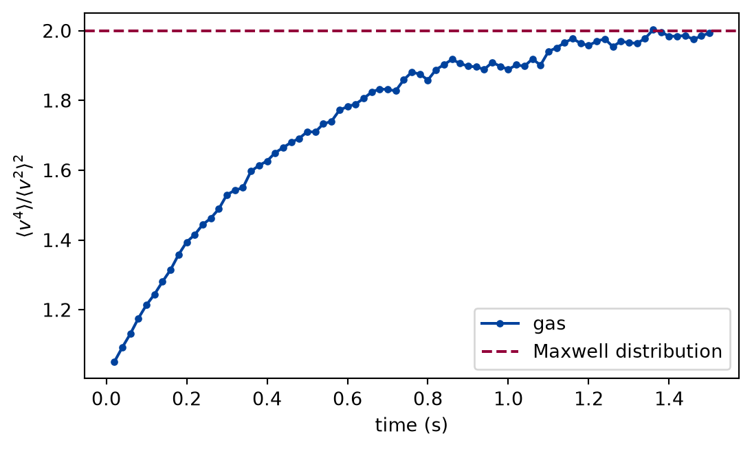
The gas has 200 discs of radius 7 mm in a box of side 1 m. They start at 1 m/s in random directions, and the time step is 2 ms, so a disc at the starting speed moves 0.14 of its diameter in one step and the packing fraction is 0.032. A first run records the ratio $\langle v^4\rangle / \langle v^2\rangle^2$ over time, averaged over twelve seeds.

SEEDS = range(12)  # twelve independent runs, fixed before they are made
THRESHOLD = 1.9  # the ratio that counts as settled; the Maxwell value is 2
# The systematic difference allowed between the model and 1 + 2 phi, on top
# of the statistical tolerance: the time step places collisions late and
# lowers the pressure, the series stops at its first correction, and the
# walls of a small box thin the gas in the middle a little.
PRESSURE_ALLOWANCE = 0.015

src/pbc/thermodynamics/experiments/particles_in_a_box.py, lines 39 to 45, read from the repository when this page was built.

def relaxation_history(experiment: Experiment):
    """Twelve runs from equal speeds, and the ratio of the moments of the speed
    over time; record the table of three moments."""
    histories = []
    for seed in SEEDS:
        start = initial_gas(N_DISCS, RADIUS, SIDE, SPEED, np.random.default_rng(seed))
        recorded = run_gas(start, 1.5, DT, EVERY)
        histories.append([speed_ratio(row) for row in recorded.speeds])
    times = recorded.times
    ratio_history = np.mean(histories, axis=0)

    assert (ratio_history > THRESHOLD).any(), "the ratio never reached the threshold"
    settled = times[np.argmax(ratio_history > THRESHOLD)]
    assert settled < RELAX, "the gas settled after the relaxation time"

    experiment.table(
        "relaxation-history",
        [
            ("start", times[0], ratio_history[0]),
            (
                "first above the threshold",
                settled,
                ratio_history[np.argmax(ratio_history > THRESHOLD)],
            ),
            ("end of the run", times[-1], ratio_history[-1]),
        ],
        [("moment", "", ""), ("time", "s", ".2f"), ("ratio of the moments", "", ".2f")],
        "The ratio of the fourth moment of the speed to the square of the second, "
        "averaged over twelve runs, at three moments of the relaxation.",
    )
    return times, ratio_history, settled

src/pbc/thermodynamics/experiments/particles_in_a_box.py, lines 76 to 106, read from the repository when this page was built.

The ratio of the fourth moment of the speed to the square of the second, averaged over twelve runs, at three moments of the relaxation.
moment	time (s)	ratio of the moments
start	0.02	1.05
first above the threshold	0.84	1.90
end of the run	1.50	1.99

def draw_relaxation(times, ratio_history) -> Figure:
    """The ratio of the moments against time."""
    fig, ax = plt.subplots(figsize=(6.4, 3.6))
    ax.plot(
        times, ratio_history, color="#00429d", marker="o", markersize=3, label="gas"
    )
    ax.axhline(2.0, color="#93003a", linestyle="--", label="Maxwell distribution")
    ax.set_xlabel("time (s)")
    ax.set_ylabel(r"$\langle v^4\rangle / \langle v^2\rangle^2$")
    ax.legend()
    return fig

src/pbc/thermodynamics/experiments/particles_in_a_box.py, lines 109 to 119, read from the repository when this page was built.

Line plot of the ratio against time in seconds. The solid line starts near one and rises quickly, then fluctuates around a dashed horizontal line at two for the rest of the time. — Figure 1: simulated The ratio of the moments starts near one, because all discs have the same speed, and reaches the Maxwell value before the measurement begins. Nothing in the rules asks for it.

Numerically verified (this gas, twelve seeds, the stated time step): Starting from one speed, the gas approaches the Maxwell value of the moment ratio, passing a ratio of 1.9, before the measurement begins. The ratio starts at 1.05, close to the one of equal speeds, and first exceeds 1.9 after 0.84 s, before the measurement begins at 1.5 s. The data are twelve simulated runs and the check is the Maxwell value, two.

The relaxed gas against kinetic theory

Now the measurement. Each of the twelve seeds runs a gas, relaxes it for 1.5 s, and measures it for the next 3.5 s.

def kinetic_theory_check(experiment: Experiment):
    """Twelve measured runs, and the rule of the lesson for their moment
    ratio and pressure against kinetic theory; record the table."""
    measurements = [measure(seed) for seed in SEEDS]

    ratio = agreement(
        [speed_ratio(m.speeds) for m in measurements],
        2.0,
        ratio_allowance(N_DISCS),
    )
    pressures = [m.pressure / m.ideal_pressure for m in measurements]
    pressure = agreement(
        pressures,
        virial_correction(measurements[0].packing_fraction),
        PRESSURE_ALLOWANCE,
    )
    ideal = agreement(pressures, 1.0, PRESSURE_ALLOWANCE)

    experiment.table(
        "kinetic-theory-check",
        [
            (
                name,
                a.mean,
                a.error,
                a.theory,
                a.difference,
                a.tolerance,
                "yes" if a.agrees else "no",
            )
            for name, a in (
                ("moment ratio", ratio),
                ("P / P_ideal", pressure),
                ("P / P_ideal against the ideal gas law alone", ideal),
            )
        ],
        [
            ("quantity", "", ""),
            ("mean over twelve runs", "", ".3f"),
            ("standard error", "", ".3f"),
            ("theory", "", ".3f"),
            ("difference", "", "+.3f"),
            ("tolerance", "", ".3f"),
            ("within the tolerance", "", ""),
        ],
        "Each quantity averaged over twelve runs, with its standard error, the "
        "theory, the difference, and the tolerance of the rule: the allowance "
        "plus the t factor times the standard error.",
    )
    return measurements, ratio, pressure, ideal

src/pbc/thermodynamics/experiments/particles_in_a_box.py, lines 122 to 171, read from the repository when this page was built.

Each quantity averaged over twelve runs, with its standard error, the theory, the difference, and the tolerance of the rule: the allowance plus the t factor times the standard error.
quantity	mean over twelve runs	standard error	theory	difference	tolerance	within the tolerance
moment ratio	1.965	0.017	2.000	-0.035	0.086	yes
P / P_ideal	1.055	0.003	1.063	-0.009	0.030	yes
P / P_ideal against the ideal gas law alone	1.055	0.003	1.000	+0.055	0.030	no

The kinetic energy is the same in every run, because the collisions and bounces conserve it and every run starts with the same.

Numerically verified (a dilute gas of hard discs in two dimensions, twelve seeds, the stated time step, the stated allowances, a false-failure probability of one in a thousand): The moment ratio of the relaxed gas agrees with the Maxwell value two, and the pressure with the virial prediction that includes the area of the discs, by the rule of the lesson; the ideal gas law alone does not. The ratio is 1.965 with a standard error of 0.017 over the twelve runs, within the tolerance of 0.086 of two. The pressure is 1.055 times that of ideal points, and the prediction with the area of the discs is 1.063, a difference of 0.009 within the tolerance of 0.030. The ideal gas law alone is off by 0.055, outside the same tolerance of 0.030, so the area of the discs matters and the check can tell the two apart. It cannot tell more: the measured pressure is somewhat below $1 + 2\varphi$ at this time step, and a difference of that size is inside the allowance.

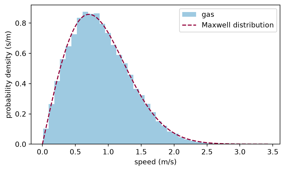
def draw_speeds(measurements) -> Figure:
    """The pooled speeds of the twelve runs against the Maxwell distribution."""
    pooled = np.concatenate([m.speeds.ravel() for m in measurements])
    kt = temperature(pooled, 1.0)
    v = np.linspace(0.0, pooled.max(), 200)

    fig, ax = plt.subplots(figsize=(6.4, 3.6))
    ax.hist(pooled, bins=40, density=True, color="#9ecae1", label="gas")
    ax.plot(
        v,
        rayleigh_pdf(v, kt, 1.0),
        color="#93003a",
        linestyle="--",
        label="Maxwell distribution",
    )
    ax.set_xlabel("speed (m/s)")
    ax.set_ylabel("probability density (s/m)")
    ax.legend()
    return fig

src/pbc/thermodynamics/experiments/particles_in_a_box.py, lines 174 to 192, read from the repository when this page was built.

Histogram of disc speeds in metres per second. The bars rise from zero at zero speed to a single peak and fall off in a long tail, and a dashed curve of the Maxwell distribution follows the tops of the bars closely. — Figure 2: simulated The pooled speeds of the twelve relaxed runs follow the Maxwell curve at the measured temperature; the agreement is judged by eye here, and by the moment ratio in the table.

The histogram pools the speeds of all discs of the twelve runs, which is allowed for a picture and not for the standard error: the discs of one run are not independent (the sixth assumption).

Limits

The checks compare two numbers with theory, within the statistical tolerance of the runs, in a model that was computed.

A model checked against a theory, not against a gas. The data are simulated. The result says that the model produces a Maxwell distribution and the virial pressure of a dilute gas. It does not say that the model is a gas of real molecules: the discs are two-dimensional, smooth, and elastic. No experiment is involved, so no claim of this lesson is experimentally supported.
What the tolerance can see. A model wrong by more than the tolerance is caught, and one wrong by less is not. The pressure check confirms the correction for the area of the discs, not its exact size: a difference from $1 + 2\varphi$ smaller than the allowance passes. One moment ratio does not fix a distribution: it is a test of the shape, not a proof of it.
The time step. The step resolves a collision only to a fraction of a diameter, and a collision is placed at the end of the step, which lowers the measured pressure by about 0.007; the allowance covers it, and a smaller step would shrink it.
The first rule in isolation. The checks do not test a single wall bounce or collision; unit tests of one bounce and one collision compare the outcome with the exact one.
Few runs, one density. Twelve runs give a standard error that is itself uncertain, which the $t$ factor allows for. The rule fails a correct model in one case in a thousand, not never. Only the density of the first example and that of the exercise are tried, and a dense gas needs more of the series.

Self-check. The moment ratio of the relaxed gas is within the tolerance of two. Does that show that the speeds follow the Maxwell distribution? What would a failure show?

With scripts, you can record in this browser that you answered this question.

Solution to the self-check

No. The ratio tests one property of the shape, the same for any distribution whose fourth moment is twice the squared second moment, and it is compared with two only to within the tolerance of twelve runs, so a distribution that differs a little is not caught. The histogram against the curve is a second, looser look. A failure would be a strong reason to look at the model or the program, not a proof against them: the rule fails a correct model in one case in a thousand, and a repeat with other seeds tells chance and error apart.

Exercises

Exercise 1. A denser gas. How many discs of the same radius give a packing fraction of 5 per cent, and what does the virial correction predict for the pressure? Run one seed of that gas and compare it with the packing fraction of the first worked example.

Solution to exercise 1

The packing fraction is $N \pi r^2 / L_\text{free}^2$ , with $L_\text{free}$ the side the centres can reach, so $N = \varphi L_\text{free}^2 / (\pi r^2)$ .

def denser_gas(experiment: Experiment) -> None:
    """Exercise 1: a gas at a packing fraction of five per cent; record the
    table."""
    free = SIDE - 2.0 * RADIUS
    n_dense = round(0.05 * free**2 / (np.pi * RADIUS**2))
    dense = measure(0, n=n_dense)
    experiment.table(
        "denser-gas",
        [
            (
                n_dense,
                dense.packing_fraction,
                virial_correction(dense.packing_fraction),
                dense.pressure / dense.ideal_pressure,
            )
        ],
        [
            ("discs", "", "d"),
            ("packing fraction", "", ".3f"),
            ("predicted P / P_ideal", "", ".3f"),
            ("measured P / P_ideal", "", ".3f"),
        ],
        "The denser gas of one seed: the number of discs, the packing fraction, and "
        "the predicted and measured pressure.",
    )

src/pbc/thermodynamics/experiments/particles_in_a_box.py, lines 195 to 219, read from the repository when this page was built.

The denser gas of one seed: the number of discs, the packing fraction, and the predicted and measured pressure.
discs	packing fraction	predicted P / P_ideal	measured P / P_ideal
316	0.050	1.100	1.079

One seed is one run, so its pressure differs from the prediction by about the spread between the runs of the table above, not by the standard error of their mean.

Exercise 2. Same seed, same gas. Run the gas of seed 0 twice and the gas of seed 1 once, each for half a second. Which of the final speeds agree?

Solution to exercise 2

The generator is created from the seed, and nothing else in the model is random, so the same seed gives the same run, bit for bit, and another seed gives another.

def final_speeds(seed):
    gas0 = initial_gas(N_DISCS, RADIUS, SIDE, SPEED, np.random.default_rng(seed))
    return run_gas(gas0, 0.5, DT, 250).speeds[-1]

src/pbc/thermodynamics/experiments/particles_in_a_box.py, lines 222 to 224, read from the repository when this page was built.

def same_seed(experiment: Experiment) -> None:
    """Exercise 2: whether two runs of one seed, and of two seeds, end with
    identical speeds; record the table."""
    first, again, other = final_speeds(0), final_speeds(0), final_speeds(1)
    experiment.table(
        "same-seed",
        [
            ("seed 0 twice", "yes" if np.array_equal(first, again) else "no"),
            ("seed 0 against seed 1", "yes" if np.array_equal(first, other) else "no"),
        ],
        [("comparison", "", ""), ("identical final speeds", "", "")],
        "Whether the final speeds of two runs are identical.",
    )

src/pbc/thermodynamics/experiments/particles_in_a_box.py, lines 227 to 239, read from the repository when this page was built.

Whether the final speeds of two runs are identical.
comparison	identical final speeds
seed 0 twice	yes
seed 0 against seed 1	no

Run this experiment

This page was built from commit 6417e2ff90258bd2d2ba21d217eb7666fd24f680 of the repository.

In a clone at that commit, with the project’s Python packages installed, this command runs the experiment of this page:

uv run --locked --no-dev python -m pbc.thermodynamics.experiments.particles_in_a_box results

Files, tests, and every command

The files behind it:

site/lessons/agents-abm/01-particles-in-a-box/index.qmd: this page, with every code cell.
src/pbc/abm/gas.py: code the experiment runs.
src/pbc/abm/acceptance.py: code the experiment runs.
src/pbc/mechanics/particles.py: code the experiment runs.
src/pbc/thermodynamics/experiments/particles_in_a_box.py: code the experiment runs.
src/pbc/experiment.py: code the experiment runs.
tests/unit/test_gas.py: tests of that code.
tests/unit/test_acceptance.py: tests of that code.
tests/unit/test_particles.py: tests of that code.
tests/unit/test_particles_in_a_box_experiment.py: tests of that code.

With Git and uv installed (see the setup page), run:

git clone https://github.com/taspinar/physics-by-construction.git
cd physics-by-construction
git checkout 6417e2ff90258bd2d2ba21d217eb7666fd24f680
uv sync --locked --no-dev
uv run --locked --no-dev python -m pbc.thermodynamics.experiments.particles_in_a_box results

The experiment writes every figure of this page into results/, as <label>.png, and every number and table of the page, as the page shows it, into results/results.json. Its numbers match this page to the digits shown, and its figure files are the ones the page shows; digits beyond those can differ between machines, because floating-point libraries differ. Change the code of the experiment and run it again to see what changes.