Momentum and collisions

Pairwise forces on the stepping interface, the total momentum that every integrator of the course then conserves to round-off, the centre of mass, and collisions as brief, strong forces whose outcome tends to the hard-sphere one.
Course
Classical mechanics, lesson 7 of 28
Slot
M7, Momentum and collisions
Methods
Simulation
Difficulty
Intermediate, level 2 of 3
What you’ll learn
  • Write pairwise forces on the stepping interface
  • Check that the total momentum is conserved to round-off
  • Model a collision as a brief strong force and compare it with the hard-sphere outcome
Prerequisites
Energy conservation.
Before you begin
  • Vectors: components, the dot product, and the unit vector along a direction
Related
Particles in a box, Momentum in a collision, proved
Previous
Energy conservation
Next
The Kepler orbit

With scripts, this page keeps a record in your browser of whether you completed the lesson. Nothing is stored without them.

With scripts, this place suggests what to do next, with the reason, from the progress saved in your browser. Without them, follow the learning path.

When a cue ball hits a rack, where does each ball go, and what does a program have to do to get it right? The question has two halves. The first is about conservation: the balls push on one another, each push has an equal and opposite partner, and so the total momentum of the balls cannot change whatever the pushes are. The second is about the contact: a collision lasts a few milliseconds, during which the force is enormous and changes quickly, and a simulation that steps through it too coarsely gets the outgoing speeds wrong. The same two questions return in every gas, every granular flow, and every molecular simulation.

Every lesson so far simulated one particle under forces that came from outside it. This lesson puts several particles on the stepping interface of the Newton’s laws lesson, with the forces between them given once per pair, and shows that the conservation of the total momentum is then not an approximation of the simulation but an identity of it, exact to round-off for every method of the course. A collision is then not a new kind of interaction but a brief, strong force: a stiff spring that pushes only while two bodies overlap. The outcome of an elastic collision between hard spheres is derived from momentum and energy alone, and the lesson measures how, and how fast, the simulated soft spheres approach it as the spring stiffens and the step shrinks with it. The many-particle gas of the agent-based modelling strand is built from these pieces.

Assumptions

The model and the program rest on these assumptions. Each one names what goes wrong when it does not hold.

  1. Forces act in pairs, and the force on one of a pair is the opposite of the force on the other. This is Newton’s third law, and it is built into the interface: a pairwise force is given once. A force that violates it, such as a magnetic force between moving charges, is not expressible here, and with it the total momentum of the particles alone is not conserved.
  2. No external force. The particles act on each other and on nothing else, so the total momentum is constant and the centre of mass moves in a straight line. With gravity or walls added, the momentum changes by the external impulse; the capstone lesson keeps the model, and the agent-based modelling strand adds the walls.
  3. The pairwise force is conservative: central, along the line between the pair, with a magnitude that depends on the distance alone, 𝑭(𝒓)=f(r)𝒓/r\mathbf F(\mathbf r) = f(r)\,\mathbf r/r. Then it has a potential energy per pair, and the total energy is the second conserved quantity. This is a stronger assumption than the interface enforces. A pairwise force is any function of the relative position, and a non-central one, such as 𝑭(𝒓)=(βˆ’y,x)\mathbf F(\mathbf r) = (-y, x), satisfies the third law and conserves momentum while doing net work around a closed path. Both pair forces of this lesson are central. A velocity-dependent contact force, which is how a real collision loses energy, is not modelled; every collision here is elastic.
  4. A collision is a Hookean contact: the repulsion grows in proportion to the overlap. This is a model, not a law. Real contacts follow stiffer, nonlinear laws and dissipate energy (not verified); the lesson models neither and has no source for them. The hard-sphere result does not depend on the contact model, and the lesson measures the distance to it, which does.
  5. The step resolves the contact. The duration of a contact is πμ/k\pi\sqrt{\mu/k}, derived below, and the step is a small fraction of it. A step comparable with the contact time gives outgoing speeds that are wrong by a large factor, as the table of the head-on collision shows, and the force has a kink where the spheres touch, so the error does not shrink smoothly with the step.
  6. Round-off is negligible. The conservation checks below are bounds far above the resolution of double precision and far below every other quantity on the page; no result is displayed at the level of round-off.

Pairs, momentum, and the centre of mass

Let nn particles with the masses mim_i be at the positions 𝒙i\mathbf x_i with the velocities 𝒗i\mathbf v_i. The force on particle ii is the sum of the forces from the others, 𝑭i=βˆ‘jβ‰ i𝑭ij\mathbf F_i = \sum_{j \ne i} \mathbf F_{ij}, and Newton’s third law says 𝑭ji=βˆ’π‘­ij\mathbf F_{ji} = -\mathbf F_{ij}. Summing the equations of motion mi𝒗̇i=𝑭im_i \dot{\mathbf v}_i = \mathbf F_i over all the particles, every pair of forces cancels, and

ddtβˆ‘imi𝒗i=βˆ‘i𝑭i=𝟎. \frac{\mathrm{d}}{\mathrm{d}t} \sum_i m_i \mathbf v_i = \sum_i \mathbf F_i = \mathbf 0 .

The total momentum 𝑷=βˆ‘imi𝒗i\mathbf P = \sum_i m_i \mathbf v_i is constant. With the total mass M=βˆ‘imiM = \sum_i m_i and the centre of mass 𝑿=1Mβˆ‘imi𝒙i\mathbf X = \tfrac{1}{M}\sum_i m_i \mathbf x_i, the total momentum is M𝑿̇M \dot{\mathbf X}: the centre of mass moves in a straight line at a constant velocity, whatever the particles do around it. For two particles the motion separates completely. Writing 𝒓=𝒙1βˆ’π’™2\mathbf r = \mathbf x_1 - \mathbf x_2 for the position of the first relative to the second, subtracting the two equations of motion gives

π’“Μˆ=𝑭12m1βˆ’π‘­21m2=(1m1+1m2)𝑭12=𝑭12ΞΌ,ΞΌ=m1m2m1+m2. \ddot{\mathbf r} = \frac{\mathbf F_{12}}{m_1} - \frac{\mathbf F_{21}}{m_2} = \Bigl(\frac{1}{m_1} + \frac{1}{m_2}\Bigr) \mathbf F_{12} = \frac{\mathbf F_{12}}{\mu}, \qquad \mu = \frac{m_1 m_2}{m_1 + m_2}.

The relative motion is that of one particle of the reduced mass ΞΌ\mu under the pair force. Two masses on a spring oscillate with Ο‰=k/ΞΌ\omega = \sqrt{k/\mu}, and the capstone lesson turns two bodies under gravity into one body about a fixed centre by the same step.

The discrete third law

The simulation conserves the total momentum exactly, not approximately, and the reason holds for every method of the course. Each integrator changes the velocities by a sum of acceleration evaluations times weights: explicit and symplectic Euler by Ξ”t𝒂(β‹…)\Delta t\,\mathbf a(\cdot), velocity Verlet by 12Ξ”t(𝒂n+𝒂n+1)\tfrac{1}{2}\Delta t\,(\mathbf a_n + \mathbf a_{n+1}), the classical Runge-Kutta method by the weighted average of four. In every evaluation the acceleration of particle ii is 𝑭i/mi\mathbf F_i / m_i with the forces of that one evaluation, which obey the third law, so βˆ‘imi𝒂i=βˆ‘i𝑭i=𝟎\sum_i m_i \mathbf a_i = \sum_i \mathbf F_i = \mathbf 0 for each evaluation separately. A weighted sum of such evaluations has a zero mass-weighted sum too, hence βˆ‘imi𝒗i\sum_i m_i \mathbf v_i is the same after the step as before it, up to round-off, for any step size and any state.

The position updates follow. Every method moves particle ii by a combination of its velocities, Δ𝒙i=Ξ”tπ’˜i+12Ξ”t2𝒃i\Delta\mathbf x_i = \Delta t\,\mathbf w_i + \tfrac12\Delta t^2\,\mathbf b_i, where π’˜i\mathbf w_i is a weighted average of velocities of the step and 𝒃i\mathbf b_i is either zero or a weighted acceleration of the step (velocity Verlet has the second term). The mass-weighted sum of the weighted accelerations is zero, as above. The mass-weighted sum of the weighted velocities is the total momentum 𝑷\mathbf P, because the momentum is the same in every stage of the step. Therefore 𝑿n+1=𝑿n+Ξ”t𝑷/M\mathbf X_{n+1} = \mathbf X_n + \Delta t\,\mathbf P/M: the simulated centre of mass moves in an exact straight line. These are the discrete counterparts of the conservation law, and they follow from the structure of the methods, not from their accuracy: explicit Euler, which cannot hold the energy of an oscillator for a single period, holds the total momentum forever.

Elastic collisions

Two hard spheres of masses m1m_1 and m2m_2 collide. The contact force acts along the line of centres, with the unit vector 𝒏\mathbf n from the second sphere to the first, so the collision changes the velocities by an impulse j𝒏j\,\mathbf n with a number jj to be found, and the components across 𝒏\mathbf n are untouched:

𝒗1β€²=𝒗1βˆ’jm1𝒏,𝒗2β€²=𝒗2+jm2𝒏. \mathbf v_1' = \mathbf v_1 - \frac{j}{m_1}\,\mathbf n, \qquad \mathbf v_2' = \mathbf v_2 + \frac{j}{m_2}\,\mathbf n .

Any jj conserves the momentum; the equal and opposite impulses are the third law. The component of the relative velocity along 𝒏\mathbf n is w=(𝒗1βˆ’π’—2)⋅𝒏w = (\mathbf v_1 - \mathbf v_2)\cdot\mathbf n, and after the collision it is wβ€²=wβˆ’j/ΞΌw' = w - j/\mu. The change of the kinetic energy of the pair is

Ξ”T=βˆ’jw+j22ΞΌ, \Delta T = -j\,w + \frac{j^2}{2\mu},

which is zero, for an elastic collision, at j=0j = 0 (no collision) and at j=2ΞΌwj = 2\mu\,w. The second root is the collision: it gives wβ€²=βˆ’ww' = -w, the component of the relative velocity along 𝒏\mathbf n reverses, and

𝒗1β€²=𝒗1βˆ’2m2m1+m2[(𝒗1βˆ’π’—2)⋅𝒏]𝒏,𝒗2β€²=𝒗2+2m1m1+m2[(𝒗1βˆ’π’—2)⋅𝒏]𝒏. \mathbf v_1' = \mathbf v_1 - \frac{2 m_2}{m_1 + m_2}\,\bigl[(\mathbf v_1 - \mathbf v_2)\cdot\mathbf n\bigr]\,\mathbf n, \qquad \mathbf v_2' = \mathbf v_2 + \frac{2 m_1}{m_1 + m_2}\,\bigl[(\mathbf v_1 - \mathbf v_2)\cdot\mathbf n\bigr]\,\mathbf n.

Three consequences. Head on with equal masses the spheres exchange velocities. A light sphere hitting a heavy one at rest has 𝒗1β€²=m1βˆ’m2m1+m2𝒗1\mathbf v_1' = \frac{m_1 - m_2}{m_1 + m_2}\mathbf v_1, which tends to βˆ’π’—1-\mathbf v_1 as m2m_2 grows. And equal spheres with one at rest give 𝒗2β€²=(𝒗1⋅𝒏)𝒏\mathbf v_2' = (\mathbf v_1\cdot\mathbf n)\mathbf n and 𝒗1β€²=𝒗1βˆ’(𝒗1⋅𝒏)𝒏\mathbf v_1' = \mathbf v_1 - (\mathbf v_1\cdot\mathbf n)\mathbf n, along and across the line of centres, so they leave at a right angle. The result does not depend on what the contact force is, only on its direction and on the energy being conserved. It is the reference the simulation is measured against.

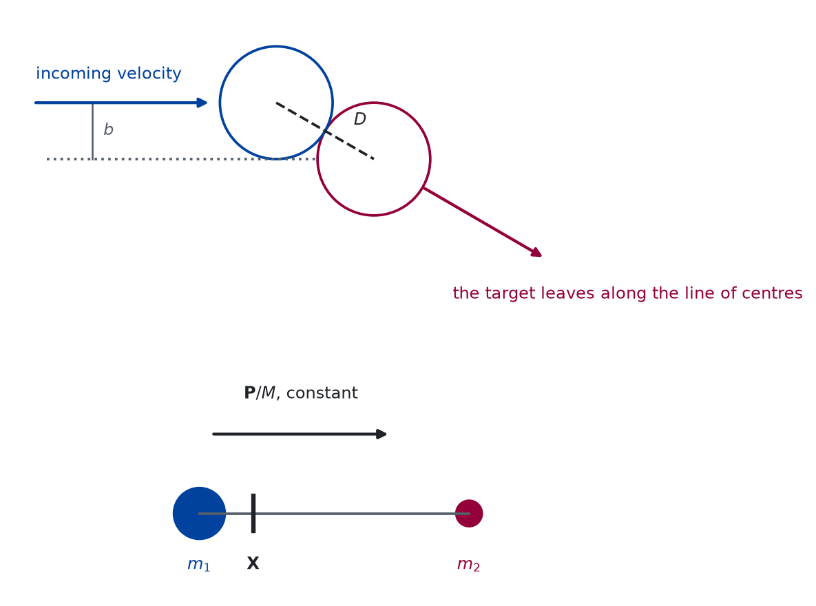
Two pictures carry the geometry of the last two sections. The upper one is a collision at first touch: the line of centres, which fixes the direction of the impulse, and the offset bb of the incoming path. The lower one is the centre of mass of two unequal masses.

def draw_collision_geometry() -> Figure:
    """The geometry of a glancing collision and the centre of mass of a pair,
    as a sketch."""
    fig, (geometry, centre) = plt.subplots(
        2, 1, figsize=(6.4, 4.8), gridspec_kw={"height_ratios": [1.5, 1]}
    )
    radius, b = 0.5, 0.5
    contact = (-np.sqrt(1.0 - b**2), b)
    diagrams.frame(geometry, (-3.2, 3.2), (-1.5, 1.3))
    diagrams.circle(geometry, (0.0, 0.0), radius, colour=1)
    diagrams.circle(geometry, contact, radius, colour=0)
    diagrams.line(geometry, [(-2.9, 0.0), (-0.5, 0.0)], colour="#57606a", linestyle=":")
    diagrams.arrow(geometry, (-3.0, b), (contact[0] - radius - 0.1, b), colour=0)
    diagrams.text(geometry, (-3.0, b + 0.25), "incoming velocity", ha="left", colour=0)
    diagrams.line(geometry, [(-2.5, 0.0), (-2.5, b)], colour="#57606a", width=1.0)
    diagrams.text(geometry, (-2.4, b / 2), "$b$", ha="left", colour="#57606a")
    diagrams.line(geometry, [contact, (0.0, 0.0)], colour="#1f2328", linestyle="--")
    diagrams.text(geometry, (-0.12, 0.34), "$D$", ha="center")
    diagrams.arrow(geometry, (0.45, -0.26), (1.5, -0.87), colour=1)
    diagrams.text(
        geometry,
        (0.7, -1.2),
        "the target leaves along the line of centres",
        ha="left",
        colour=1,
    )
    diagrams.frame(centre, (-0.4, 5.4), (-1.0, 1.9))
    diagrams.line(centre, [(0.3, 0.0), (3.7, 0.0)], colour="#57606a")
    diagrams.circle(centre, (0.3, 0.0), 0.32, colour=0, filled=True)
    diagrams.circle(centre, (3.7, 0.0), 0.16, colour=1, filled=True)
    diagrams.text(centre, (0.3, -0.65), "$m_1$", colour=0)
    diagrams.text(centre, (3.7, -0.65), "$m_2$", colour=1)
    com = 0.3 + 3.4 * 0.2
    diagrams.line(centre, [(com, -0.22), (com, 0.22)], colour="#1f2328", width=2.4)
    diagrams.text(centre, (com, -0.65), "$\\mathbf{X}$", colour="#1f2328")
    diagrams.arrow(centre, (com - 0.5, 1.0), (com + 1.7, 1.0), colour="#1f2328")
    diagrams.text(
        centre, (com + 0.6, 1.5), "$\\mathbf{P}/M$, constant", colour="#1f2328"
    )
    fig.tight_layout()
    return fig
src/pbc/mechanics/experiments/momentum_and_collisions.py, lines 81 to 121, read from the repository when this page was built.

Two diagrams. The upper one shows two circles touching. A blue circle comes in from the left along a horizontal arrow that lies a distance b above the horizontal through the centre of a red circle. A dashed line joins the two centres, and a red arrow leaves the red circle along that line, down and to the right. The lower one shows a large blue dot and a small red dot joined by a line, a tick mark for the centre of mass close to the large dot, and an arrow above it pointing right for the constant velocity.
Figure 1: conceptual Above, a collision at first touch: the moving sphere, blue, comes in along a path that misses the centre of the target by the offset b, the centres are a distance D apart, and the target leaves along the line of centres. Below, the centre of mass of two unequal masses lies on the line between them, nearer the heavy one, and moves at the constant velocity that the total momentum fixes.

Both are sketches. The upper answers why the offset decides the angle: the impulse acts along the line of centres, so only the offset sets its direction. The lower answers why the centre of mass is a useful frame: the internal forces cancel in pairs, so whatever the particles do, the point moves in a straight line.

The soft-sphere model

The simulation needs a force, and the simplest one that acts only on contact is a spring that pushes while the spheres overlap: with DD the sum of the two radii and r=|𝒓|r = |\mathbf r| the distance between the centres,

𝑭12={k(Dβˆ’r)𝒓rr<D,𝟎rβ‰₯D. \mathbf F_{12} = \begin{cases} k\,(D - r)\,\dfrac{\mathbf r}{r} & r < D, \\[1ex] \mathbf 0 & r \ge D . \end{cases}

In a head-on collision the overlap is Ξ΄=Dβˆ’r\delta = D - r, and the relative motion obeys r̈=F12/ΞΌ\ddot r = F_{12}/\mu with F12=kΞ΄F_{12} = k\delta, so μδ̈=βˆ’kΞ΄\mu\,\ddot\delta = -k\,\delta. At first touch Ξ΄=0\delta = 0 and Ξ΄Μ‡=u\dot\delta = u, the speed of approach, so Ξ΄(t)=(u/Ο‰)sin⁑ωt\delta(t) = (u/\omega)\sin\omega t with Ο‰=k/ΞΌ\omega = \sqrt{k/\mu}. The overlap returns to zero at Ο‰t=Ο€\omega t = \pi, where Ξ΄Μ‡=βˆ’u\dot\delta = -u: the contact is half a period of a harmonic oscillator with the reduced mass, it ends with the relative speed exactly reversed, as for hard spheres, and its duration, the contact time, is

Ο„=πμk, \tau = \pi\sqrt{\frac{\mu}{k}} ,

independent of the speed. The largest overlap is u/Ο‰u/\omega, which must be smaller than DD for the spheres to turn before their centres meet; the first exercise tests that bound. Off centre, the line of centres turns during the contact, and the soft spheres leave in a direction that differs from the hard-sphere one; the worked example below measures how that difference depends on Ο„\tau. A stiffer spring is a shorter contact and a closer approach to the hard-sphere result, and it needs a proportionally smaller step: the cost of the limit is the number of steps. The potential energy of the contact is 12kΞ΄2\tfrac{1}{2} k\,\delta^2 while the spheres overlap, so the total energy of the pair is conserved through the collision, and its drift is the diagnostic of the previous lesson on a force with a kink.

The program

The reusable code lives in the module pbc.mechanics.particles of the repository. It runs several particles on the single-particle interface of the Newton’s laws lesson, so simulate and the four steppers are the ones of the earlier lessons, unchanged. The listings in this section are read from the file when the site is built.

The state of nn particles in dd dimensions is one vector of length ndn d; two helpers convert between it and one row per particle:

def stack(rows: ArrayLike) -> Vector:
    """The positions or velocities of n particles, one row each, as the one
    vector of length n d that the state of the system holds."""
    return np.array(rows, dtype=np.float64, ndmin=2).reshape(-1)

src/pbc/mechanics/particles.py, lines 34 to 37, read from the repository when this page was built.

def unstack(flat: ArrayLike, n: int) -> NDArray[np.float64]:
    """The vector of length n d back to one row per particle, shape (n, d);
    an array of such vectors, such as the positions of a trajectory with
    shape (steps, n d), becomes an array of shape (steps, n, d)."""
    if n <= 0:
        raise ValueError(f"the number of particles must be positive, got {n}")
    array = np.array(flat, dtype=np.float64)
    if array.shape[-1] % n:
        raise ValueError(
            f"a vector of length {array.shape[-1]} does not hold {n} particles"
        )
    return array.reshape(*array.shape[:-1], n, -1)

src/pbc/mechanics/particles.py, lines 40 to 51, read from the repository when this page was built.

The acceleration of the system from the masses and one pairwise force. The order of the two updates inside the double loop is where the third law, and with it the conservation of the momentum, is built in:

def interacting(masses: ArrayLike, pairwise: PairwiseForce) -> Acceleration:
    """The acceleration of n particles with the given ``masses`` (kg) that act
    on one another through the ``pairwise`` force.

    For every pair the force on the first particle is ``pairwise`` of its
    position relative to the second, and the second feels the opposite, so
    the forces sum to zero over the system. The acceleration of each
    particle is the sum of the forces on it divided by its mass. The state
    is the stacked vector of ``stack``.
    """
    m = _masses(masses)
    n = len(m)

    def acceleration(t: float, x: Vector, v: Vector) -> Vector:
        positions = unstack(x, n)
        forces = np.zeros_like(positions)
        for i in range(n):
            for j in range(i + 1, n):
                force = pairwise(positions[i] - positions[j])
                forces[i] += force
                forces[j] -= force
        return (forces / m[:, np.newaxis]).reshape(-1)

    return acceleration
  1. Line 79, force = pairwise(positions[i] - positions[j]): The force on the first particle of the pair, from its position relative to the second. It is computed once per pair.
  2. Line 80, forces[i] += force: The first particle receives the force.
  3. Line 81, forces[j] -= force: The second particle receives exactly the opposite force, the same array with its sign changed. Every force added to one particle is subtracted from another, so the forces sum to zero in every evaluation.
  4. Line 82, return (forces / m[:, np.newaxis]).reshape(-1): Only now are the forces divided by the masses, in newtons per kilogram, so the mass-weighted sum of the accelerations is the sum of the forces, which is zero.

src/pbc/mechanics/particles.py, lines 61 to 84, read from the repository when this page was built.

The quantities of the whole system, with the masses of the particles:

def centre_of_mass(masses: ArrayLike, positions: ArrayLike) -> NDArray[np.float64]:
    """The centre of mass (sum of m_i x_i) / (sum of m_i) of particles with
    the given ``masses``, for ``positions`` with one row per particle; an
    array of such rows, shape (steps, n, d), gives one centre per step."""
    m = _masses(masses)
    weighted = np.tensordot(
        np.asarray(positions, dtype=np.float64), m, axes=([-2], [0])
    )
    return weighted / m.sum()

src/pbc/mechanics/particles.py, lines 87 to 95, read from the repository when this page was built.

def total_momentum(masses: ArrayLike, velocities: ArrayLike) -> NDArray[np.float64]:
    """The total momentum, the sum of m_i v_i in kg m/s, for ``velocities``
    with one row per particle, or one such array per step."""
    m = _masses(masses)
    return np.tensordot(np.asarray(velocities, dtype=np.float64), m, axes=([-2], [0]))

src/pbc/mechanics/particles.py, lines 98 to 102, read from the repository when this page was built.

def kinetic_energy(masses: ArrayLike, velocities: ArrayLike) -> NDArray[np.float64]:
    """The kinetic energy, the sum of m_i |v_i|Β² / 2 in J, for ``velocities``
    with one row per particle, or one value per step for an array of
    them."""
    m = _masses(masses)
    speeds_squared = np.sum(np.asarray(velocities, dtype=np.float64) ** 2, axis=-1)
    return 0.5 * speeds_squared @ m

src/pbc/mechanics/particles.py, lines 105 to 111, read from the repository when this page was built.

def reduced_mass(m1: float, m2: float) -> float:
    """The reduced mass m1 m2 / (m1 + m2) in kg of a pair: the mass whose
    motion under the pair force is the relative motion of the two."""
    m = _masses([m1, m2])
    return float(m[0] * m[1] / m.sum())

src/pbc/mechanics/particles.py, lines 114 to 118, read from the repository when this page was built.

The two pair forces of this lesson, the potential of the contact, and the energy of a system of pairs:

def spring_pair(k: float, rest_length: float) -> PairwiseForce:
    """A spring with the constant ``k`` (N/m) and the ``rest_length`` (m)
    between two particles: the force -k (|r| - L_0) r / |r| on the first,
    along the line between them, pulling when the spring is stretched and
    pushing when it is compressed."""
    if k <= 0:
        raise ValueError(f"the spring constant must be positive, got {k}")
    if rest_length < 0:
        raise ValueError(f"the rest length must not be negative, got {rest_length}")

    def force(r: Vector) -> Vector:
        distance = np.sqrt(r @ r)
        return -k * (distance - rest_length) * r / distance

    return force

src/pbc/mechanics/particles.py, lines 121 to 135, read from the repository when this page was built.

def soft_sphere(k: float, diameter: float) -> PairwiseForce:
    """Two spheres that repel only while they overlap, with the force
    k (D - |r|) r / |r| on the first for |r| < D and no force otherwise:
    a spring of stiffness ``k`` (N/m) that acts only in compression, with
    ``diameter`` D the sum of the two radii (m).

    A head-on collision under this force lasts pi sqrt(mu / k) with mu the
    reduced mass of the pair and ends as the hard-sphere collision of
    ``hard_sphere_collision``, provided the spheres turn before their
    centres meet: the relative speed u must satisfy |u| sqrt(mu / k) < D,
    the relative kinetic energy below k DΒ² / 2. Faster pairs carry enough
    kinetic energy to cross the finite potential barrier k DΒ² / 2 and pass
    through each other: once the centres cross, r reverses, the repulsion
    reverses with it and now drives the pair apart, vanishing only when they
    cease to overlap. A simulation must resolve the contact time; as k grows
    the contact shortens and the outcome tends to the hard-sphere one.
    """
    if k <= 0:
        raise ValueError(f"the stiffness must be positive, got {k}")
    if diameter <= 0:
        raise ValueError(f"the diameter must be positive, got {diameter}")

    def force(r: Vector) -> Vector:
        distance = np.sqrt(r @ r)
        if distance >= diameter:
            return np.zeros_like(r)
        return k * (diameter - distance) * r / distance

    return force

src/pbc/mechanics/particles.py, lines 138 to 166, read from the repository when this page was built.

def soft_sphere_potential(k: float, diameter: float) -> PairwisePotential:
    """The energy k (D - |r|)Β² / 2 stored in the compression of two soft
    spheres that overlap, and 0 when they do not: the potential of
    ``soft_sphere``. During a collision the kinetic energy the pair loses
    is held here and given back."""
    if k <= 0:
        raise ValueError(f"the stiffness must be positive, got {k}")
    if diameter <= 0:
        raise ValueError(f"the diameter must be positive, got {diameter}")

    def potential(r: Vector) -> float:
        distance = np.sqrt(r @ r)
        return (
            float(0.5 * k * (diameter - distance) ** 2) if distance < diameter else 0.0
        )

    return potential

src/pbc/mechanics/particles.py, lines 225 to 241, read from the repository when this page was built.

def pair_potential_energy(
    positions: ArrayLike, potential: PairwisePotential
) -> NDArray[np.float64]:
    """The potential energy of a system, the sum of U(x_i - x_j) over its
    pairs, for ``positions`` with one row per particle, or one value per
    step for an array of them with shape (steps, n, d)."""
    array = np.array(positions, dtype=np.float64)
    if array.ndim == 2:
        n = array.shape[0]
        return np.array(
            sum(
                potential(array[i] - array[j])
                for i in range(n)
                for j in range(i + 1, n)
            ),
            dtype=np.float64,
        )
    return np.array([pair_potential_energy(rows, potential) for rows in array])

src/pbc/mechanics/particles.py, lines 244 to 261, read from the repository when this page was built.

The hard-sphere result to compare with, and the moment and direction of first contact for two spheres on straight paths:

def hard_sphere_collision(
    m1: float, v1: Vector, m2: float, v2: Vector, normal: Vector
) -> tuple[Vector, Vector]:
    """The velocities after an elastic collision of two hard spheres.

    ``normal`` is the unit vector along the line of centres at contact, from
    the second sphere to the first. Momentum and kinetic energy are
    conserved, and the impulse acts along the normal, so the component of
    the relative velocity along the normal reverses and the components
    across it are unchanged:

        v1' = v1 - 2 m2 / (m1 + m2) ((v1 - v2) . n) n,
        v2' = v2 + 2 m1 / (m1 + m2) ((v1 - v2) . n) n.

    Head on, with equal masses, the spheres exchange velocities.
    """
    m = _masses([m1, m2])
    v1 = np.array(v1, dtype=np.float64, ndmin=1)
    v2 = np.array(v2, dtype=np.float64, ndmin=1)
    n = np.array(normal, dtype=np.float64, ndmin=1)
    approach = (v1 - v2) @ n
    return (
        v1 - 2.0 * m[1] / m.sum() * approach * n,
        v2 + 2.0 * m[0] / m.sum() * approach * n,
    )
  1. Line 213, approach = (v1 - v2) @ n: The component of the relative velocity along the line of centres, the number called w in the derivation. Only this component changes.
  2. Line 215, v1 - 2.0 * m[1] / m.sum() * approach * n,: The first sphere loses a share of the approach speed that is larger when the other sphere is heavier.
  3. Line 216, v2 + 2.0 * m[0] / m.sum() * approach * n,: The second sphere gains the opposite impulse divided by its own mass, so the total momentum is unchanged.

src/pbc/mechanics/particles.py, lines 193 to 217, read from the repository when this page was built.

def first_contact(r: Vector, u: Vector, diameter: float) -> tuple[float, Vector]:
    """When two spheres on straight paths first touch, and how.

    ``r`` is the position of the first sphere relative to the second (m) and
    ``u`` its velocity relative to the second (m/s), both now; ``diameter``
    is the sum of the radii. Returns the time until |r + u t| = diameter and
    the unit vector along the line of centres at that moment, from the
    second sphere to the first. Raises ``ValueError`` when the spheres
    already overlap or never meet.
    """
    r = np.array(r, dtype=np.float64, ndmin=1)
    u = np.array(u, dtype=np.float64, ndmin=1)
    if r @ r <= diameter**2:
        raise ValueError("the spheres already overlap")
    # |r + u t|Β² = DΒ²: a quadratic in t; the smaller root is the first touch.
    a, b, c = u @ u, 2.0 * (r @ u), r @ r - diameter**2
    discriminant = b**2 - 4.0 * a * c
    if a == 0 or discriminant < 0 or b >= 0:
        raise ValueError("the spheres never meet")
    t = (-b - np.sqrt(discriminant)) / (2.0 * a)
    contact = r + u * t
    return float(t), contact / diameter

src/pbc/mechanics/particles.py, lines 169 to 190, read from the repository when this page was built.

Worked examples

Two masses on a spring

Two masses joined by a spring, drifting across the plane, are the simplest system with an internal force and a total momentum. The setup is given in the cell: the spring starts stretched, and the relative velocity is along the spring, so the pair does not rotate.

masses = [1.0, 3.0]  # kg
k = 12.0  # N/m
rest_length = 1.0  # m
stretch0 = 0.2  # m, how far the spring starts stretched
dt = 0.01  # s
duration = 4.0  # s
tolerance = 1e-12  # the bound the conservation checks are compared with
mu = reduced_mass(*masses)
omega = np.sqrt(k / mu)
pair = interacting(masses, spring_pair(k, rest_length))
start = State(
    t=0.0,
    x=stack([[0.0, 0.0], [rest_length + stretch0, 0.0]]),
    v=stack([[1.0, 0.5], [0.6, 0.5]]),  # relative velocity along the spring
)

src/pbc/mechanics/experiments/momentum_and_collisions.py, lines 42 to 56, read from the repository when this page was built.

The two masses are 1 kg and 3 kg, joined by a spring of 12 N/m and rest length 1 m, stretched by 0.2 m at the start. The reduced mass is 0.75 kg, so the relative motion oscillates with Ο‰=\omega = 4.0 rad/s, a period of 1.5708 s. The next cell runs 4 s with every method at a step of 0.01 s and checks the total momentum and the centre of mass against a bound of 1e-12, relative to the size of the momentum and in metres for the centre of mass: the values themselves are at the level of round-off, which differs from machine to machine and is not displayed.

def pair_conservation(experiment: Experiment) -> None:
    """The total momentum of the pair on a spring and the two conservation
    checks, for each method; record the table."""
    rows = []
    for integrator in INTEGRATORS:
        trajectory = simulate(
            start, pair, dt, round(duration / dt), step=integrator.step
        )
        positions, velocities = unstack(trajectory.x, 2), unstack(trajectory.v, 2)
        momentum = total_momentum(masses, velocities)
        centre = centre_of_mass(masses, positions)
        on_the_line = centre[0] + trajectory.t[:, np.newaxis] * momentum[0] / sum(
            masses
        )
        kept = np.max(np.abs(momentum - momentum[0])) < tolerance * np.linalg.norm(
            momentum[0]
        )
        straight = np.max(np.abs(centre - on_the_line)) < tolerance
        rows.append(
            (
                integrator.name,
                momentum[0, 0],
                momentum[0, 1],
                "yes" if kept else "no",
                "yes" if straight else "no",
            )
        )

    experiment.table(
        "pair-conservation",
        rows,
        columns=[
            ("method", "", ""),
            ("total momentum, x", "kg m/s", ".1f"),
            ("total momentum, y", "kg m/s", ".1f"),
            ("constant within the bound", "", ""),
            ("centre of mass on its line within the bound", "", ""),
        ],
        caption="The total momentum of the pair and the two conservation checks, "
        "for each method, over the whole run.",
    )

src/pbc/mechanics/experiments/momentum_and_collisions.py, lines 124 to 164, read from the repository when this page was built.

The total momentum of the pair and the two conservation checks, for each method, over the whole run.
method total momentum, x (kg m/s) total momentum, y (kg m/s) constant within the bound centre of mass on its line within the bound
explicit Euler 2.8 2.0 yes yes
symplectic Euler 2.8 2.0 yes yes
velocity Verlet 2.8 2.0 yes yes
Runge-Kutta 4 2.8 2.0 yes yes

Numerically verified (two particles, a spring, the step shown): Every method conserves the total momentum and keeps the centre of mass on its straight line within the bound, explicit Euler included. This is the discrete third law at work: the table checks it for four methods whose accuracy differs by orders of magnitude, and it does not use the accuracy at all. The relative motion is the harmonic oscillator of the reduced mass; the next cell compares the stretch of the spring with the exact motion of that oscillator, released from the same stretch with the relative velocity of the pair.

def relative_motion():
    """The pair with Runge-Kutta 4, and the largest difference between the
    stretch of the spring and the oscillator of the reduced mass, in m."""
    trajectory = simulate(start, pair, dt, round(duration / dt), step=rk4.step)
    positions = unstack(trajectory.x, 2)
    stretch = np.linalg.norm(positions[:, 1] - positions[:, 0], axis=1) - rest_length
    relative_velocity = (unstack(start.v, 2)[1] - unstack(start.v, 2)[0])[0]
    relative = harmonic_motion(
        State(t=0.0, x=[stretch0], v=[relative_velocity]), mu, k, trajectory.t
    )
    oscillator_error = np.max(np.abs(stretch - relative.x[:, 0]))
    return positions, oscillator_error

src/pbc/mechanics/experiments/momentum_and_collisions.py, lines 167 to 178, read from the repository when this page was built.

The largest difference between the stretch and the oscillator is 6.6e-08 m for the fourth-order method at this step, Numerically verified (spring pair, fourth-order method): which shows that the two-particle simulation reproduces the one-particle problem of the reduced mass.

def draw_pair_on_a_spring(positions) -> Figure:
    """The paths of the two masses and of their centre of mass."""
    centre = centre_of_mass(masses, positions)
    fig, ax = plt.subplots(figsize=(6.4, 3.6))
    for i, (label, style) in enumerate(
        ((f"{masses[0]:g} kg", "-"), (f"{masses[1]:g} kg", "--"))
    ):
        ax.plot(
            positions[:, i, 0],
            positions[:, i, 1],
            color="#93003a",
            linestyle=style,
            label=label,
        )
        ax.plot(
            positions[::50, i, 0],
            positions[::50, i, 1],
            color="#93003a",
            marker="o",
            markersize=3,
            linestyle="none",
        )
    ax.plot(
        centre[:, 0],
        centre[:, 1],
        color="#00429d",
        linestyle=":",
        label="centre of mass",
    )
    ax.set_xlabel("x (m)")
    ax.set_ylabel("y (m)")
    ax.set_aspect("equal")
    ax.legend(loc="upper left")
    return fig

src/pbc/mechanics/experiments/momentum_and_collisions.py, lines 181 to 214, read from the repository when this page was built.

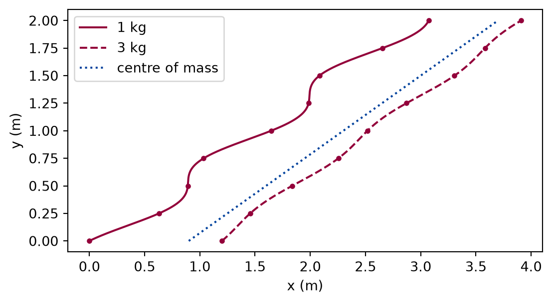
Plot of y against x in metres. Two wavy paths run from left to right, one for each mass, oscillating towards and away from each other about a straight dotted line, the centre of mass, which lies closer to the heavier path than to the lighter one. Dots along each path mark equal time intervals.
Figure 2: simulated The centre of mass moves in a straight line while the lighter mass swings through a larger path than the heavier one around it, in the ratio of the masses; the positions are marked at equal time intervals.

The paths are the fourth-order simulation of the cell above. Seen from the centre of mass, each mass swings about it by an amount inversely proportional to its mass: the centre lies 3 times closer to the heavier mass than to the lighter one, as 𝑿=βˆ‘mi𝒙i/M\mathbf X = \sum m_i \mathbf x_i / M says. The dotted line is straight, as the table checked.

A head-on collision

A sphere meets a heavier one moving towards it; the numbers are set in the cell, and the paragraph after it states them. The table the cell builds shows the outcome for hard spheres and for soft spheres run with velocity Verlet at a fixed number of steps per contact.

m1, m2 = 1.0, 2.0  # kg
v1, v2 = 1.0, -0.5  # m/s, head on along a line
diameter = 0.2  # m, the sum of the radii
stiffness = 1000.0  # N/m
fine = 40  # steps per contact for the main run
contact_time = np.pi * np.sqrt(reduced_mass(m1, m2) / stiffness)
expected = hard_sphere_collision(m1, [v1], m2, [v2], [-1.0])  # heavier one ahead
collision = interacting([m1, m2], soft_sphere(stiffness, diameter))
contact = soft_sphere_potential(stiffness, diameter)
approaching = State(t=0.0, x=stack([[0.0], [1.0]]), v=stack([[v1], [v2]]))

src/pbc/mechanics/experiments/momentum_and_collisions.py, lines 60 to 69, read from the repository when this page was built.

def collide(steps_per_contact, duration=1.2):
    """The collision, resolved with that many steps per contact time."""
    step = contact_time / steps_per_contact
    return simulate(
        approaching, collision, step, round(duration / step), step=verlet.step
    )

src/pbc/mechanics/experiments/momentum_and_collisions.py, lines 217 to 222, read from the repository when this page was built.

def head_on(experiment: Experiment):
    """The head-on collision at forty steps per contact against the elastic
    formula; record the table and return the run, its positions and
    velocities, and when the spheres first and last overlap, in s."""
    trajectory = collide(fine)
    positions, velocities = unstack(trajectory.x, 2), unstack(trajectory.v, 2)
    overlapping = positions[:, 1, 0] - positions[:, 0, 0] < diameter
    first, last = trajectory.t[overlapping][0], trajectory.t[overlapping][-1]

    experiment.table(
        "head-on",
        [
            ("hard spheres", expected[0][0], expected[1][0]),
            ("soft spheres", velocities[-1, 0, 0], velocities[-1, 1, 0]),
        ],
        columns=[
            ("model", "", ""),
            ("outgoing velocity, first sphere", "m/s", "+.4f"),
            ("outgoing velocity, second sphere", "m/s", "+.4f"),
        ],
        caption="Outgoing velocities of the head-on collision, to four decimals: "
        "the elastic formula and the simulation.",
    )
    return trajectory, positions, velocities, first, last

src/pbc/mechanics/experiments/momentum_and_collisions.py, lines 225 to 248, read from the repository when this page was built.

Outgoing velocities of the head-on collision, to four decimals: the elastic formula and the simulation.
model outgoing velocity, first sphere (m/s) outgoing velocity, second sphere (m/s)
hard spheres -1.0000 +0.5000
soft spheres -1.0000 +0.5000

The two spheres have the masses 1 kg and 2 kg, the speeds 1 m/s and 0.5 m/s towards each other, a combined diameter of 0.2 m, and a contact stiffness of 1000 N/m. The contact time is 0.0811 s; the simulated spheres overlap from 0.533 s to 0.612 s, which is the contact time to within a step. Numerically verified (head on, this stiffness, the step shown): The soft spheres leave with the hard-sphere velocities to the digits shown: the formula of the explanation and the simulation, which does not use it, agree.

def draw_head_on_collision(trajectory, positions, velocities) -> Figure:
    """The positions and the energies of the head-on collision."""
    energies = kinetic_energy([m1, m2], velocities)
    stored = pair_potential_energy(positions, contact)

    fig, (top, bottom) = plt.subplots(2, 1, figsize=(6.4, 5.2), sharex=True)
    top.plot(
        trajectory.t, positions[:, 0, 0], color="#93003a", label=f"{m1:g} kg sphere"
    )
    top.plot(
        trajectory.t,
        positions[:, 1, 0],
        color="#00429d",
        linestyle="--",
        label=f"{m2:g} kg sphere",
    )
    top.set_ylabel("position (m)")
    top.legend(loc="upper left")
    bottom.plot(trajectory.t, energies, color="#93003a", label="kinetic")
    bottom.plot(trajectory.t, stored, color="#00429d", linestyle="--", label="contact")
    bottom.plot(
        trajectory.t, energies + stored, color="#555555", linestyle=":", label="total"
    )
    bottom.set_xlabel("time (s)")
    bottom.set_ylabel("energy (J)")
    bottom.legend(loc="center left")
    fig.tight_layout()
    return fig
src/pbc/mechanics/experiments/momentum_and_collisions.py, lines 251 to 278, read from the repository when this page was built.

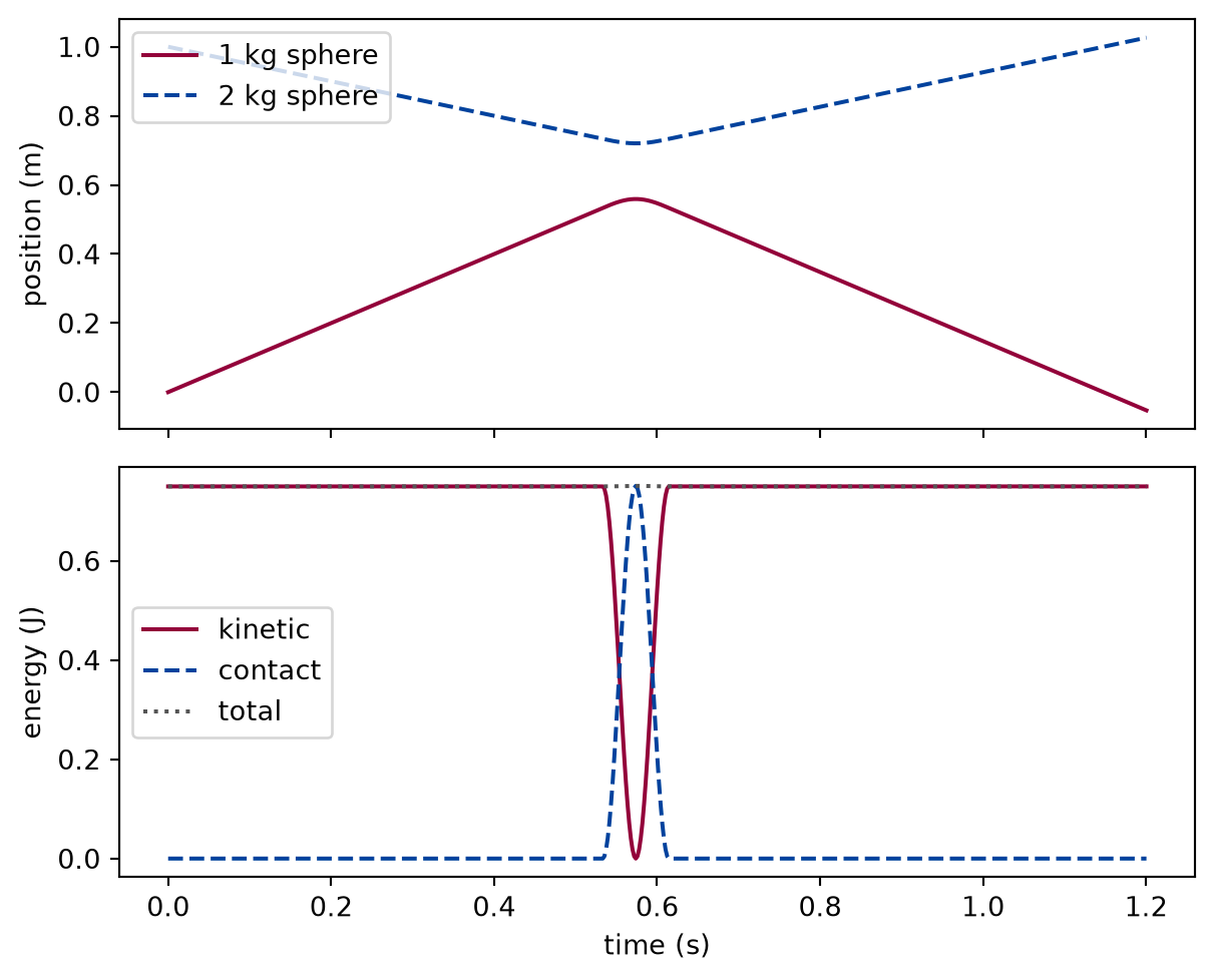
Two panels sharing the time axis in seconds. Top: the position of each sphere in metres; the two lines approach, meet, and separate at reversed slopes. Bottom: the kinetic energy dips sharply during the brief contact while the contact energy rises by the same amount in a bump; the total energy stays a flat line throughout.
Figure 3: simulated During the brief contact the kinetic energy of the pair is lent to the compression and given back, while the total stays flat; the spheres leave with reversed relative velocity.

The energies are the kinetic energy of the simulated velocities and the potential 12kΞ΄2\tfrac12 k\delta^2 of the contact, and the flat total is the check that the soft sphere is a conservative force. The step was chosen against the contact time; the next cell shows what happens to the result when it is not, with the drift of the total energy compared with the band of the numerical integrators lesson, Ο‰2Ξ”t2/4\omega^2\Delta t^2/4, in which ωΔt=Ο€/N\omega\Delta t = \pi/N for NN steps per contact.

def steps_per_contact(experiment: Experiment):
    """The head-on collision at eight step sizes; record the table and return
    the errors by steps per contact and how close the drift comes to the
    band from twenty steps on."""
    rows = []
    for steps_per_contact in (1, 2, 5, 10, 20, 40, 80, 160):
        trajectory = collide(steps_per_contact)
        positions, velocities = unstack(trajectory.x, 2), unstack(trajectory.v, 2)
        total = kinetic_energy([m1, m2], velocities) + pair_potential_energy(
            positions, contact
        )
        momentum = total_momentum([m1, m2], velocities)
        error = max(
            abs(velocities[-1, 0, 0] - expected[0][0]),
            abs(velocities[-1, 1, 0] - expected[1][0]),
        )
        drift = np.max(np.abs(total / total[0] - 1))
        band = (np.pi / steps_per_contact) ** 2 / 4
        kept = (
            np.max(np.abs(momentum - momentum[0])) < tolerance * abs(momentum[0, 0])
            if momentum[0, 0]
            else True
        )
        rows.append(
            (
                steps_per_contact,
                velocities[-1, 0, 0],
                velocities[-1, 1, 0],
                error,
                drift,
                band,
                "yes" if kept else "no",
            )
        )
    errors = {row[0]: row[3] for row in rows}
    close = [abs(row[4] / row[5] - 1) for row in rows if row[0] >= 20]

    experiment.table(
        "steps-per-contact",
        rows,
        columns=[
            ("steps per contact", "", "d"),
            ("outgoing velocity, first sphere", "m/s", ".5f"),
            ("outgoing velocity, second sphere", "m/s", ".5f"),
            ("error against hard spheres", "m/s", ".1e"),
            ("total energy drift", "", ".1e"),
            ("band", "", ".1e"),
            ("momentum constant within the bound", "", ""),
        ],
        caption="The head-on collision at eight step sizes: outgoing velocities, "
        "the larger error against the hard-sphere velocities, the largest "
        "relative drift of the total energy, and the band from the oscillator.",
    )
    return errors, close

src/pbc/mechanics/experiments/momentum_and_collisions.py, lines 281 to 334, read from the repository when this page was built.

The head-on collision at eight step sizes: outgoing velocities, the larger error against the hard-sphere velocities, the largest relative drift of the total energy, and the band from the oscillator.
steps per contact outgoing velocity, first sphere (m/s) outgoing velocity, second sphere (m/s) error against hard spheres (m/s) total energy drift band momentum constant within the bound
1 -3.19477 1.59739 2.2e+00 9.2e+00 2.5e+00 yes
2 -1.09739 0.54869 9.7e-02 7.9e-01 6.2e-01 yes
5 -1.01196 0.50598 1.2e-02 5.7e-02 9.9e-02 yes
10 -1.00095 0.50048 9.5e-04 1.8e-02 2.5e-02 yes
20 -0.99999 0.50000 5.4e-06 6.1e-03 6.2e-03 yes
40 -1.00003 0.50002 3.1e-05 1.5e-03 1.5e-03 yes
80 -1.00000 0.50000 3.9e-06 3.8e-04 3.9e-04 yes
160 -1.00000 0.50000 4.9e-07 9.5e-05 9.6e-05 yes

With one step per contact the spheres leave at the wrong speeds by a large factor, and with two the first sphere is off by 10 per cent. With five steps per contact the outgoing speeds are off by 1.2 per cent, and with ten by 0.10 per cent. Numerically verified (head on, velocity Verlet, this stiffness): The error shrinks with the step, but not smoothly: the force has a kink where the spheres touch, and where the step lands relative to it changes from one row to the next. The drift of the total energy is smoother, because during the contact the force is a plain spring: Numerically verified (from twenty steps per contact): from twenty steps per contact on, the drift lies within 1.2 per cent of the band, while the coarser rows are outside that agreement, where the kink matters most. The momentum is constant within the bound in every row, even where the outgoing speeds are badly wrong, which the self-check below uses. The step that resolves a collision is a fraction of the contact time, whatever the spheres do between collisions, and the cost of a gas simulation follows from it.

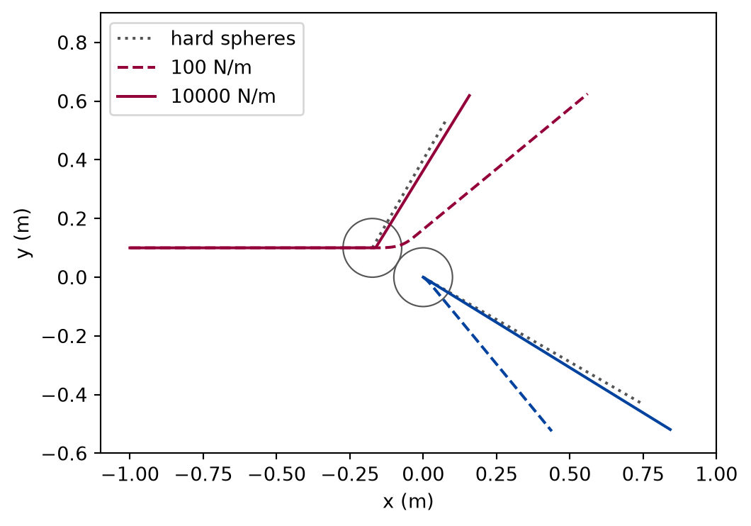
Off centre, and the hard-sphere limit

Two equal spheres with the combined diameter of the head-on collision. One is at rest; the other approaches along a line that misses the centre of the first by half the diameter. For hard spheres the geometry fixes the line of centres at contact. The moving sphere comes in along the xx axis with its centre at height bb above the other’s, and at first touch the centres are a distance DD apart, so the line of centres makes the angle Ξ±=arcsin⁑(b/D)\alpha = \arcsin(b/D) with the incoming velocity. The impulse acts along that line, and for equal masses and a target at rest the formulas of the explanation send the target along the line of centres and the moving sphere across it, so the moving sphere is deflected by 90βˆ˜βˆ’Ξ±90^\circ - \alpha and the two leave at a right angle. The cell computes these, and runs the collision with five contact stiffnesses, each with the same number of steps per contact as before.

offset = 0.1  # m, the distance by which the path misses the centre

src/pbc/mechanics/experiments/momentum_and_collisions.py, line 73, read from the repository when this page was built.

def angle_between(u, w):
    return np.degrees(np.arccos(u @ w / (np.linalg.norm(u) * np.linalg.norm(w))))

src/pbc/mechanics/experiments/momentum_and_collisions.py, lines 337 to 338, read from the repository when this page was built.

def glancing_sweep():
    """The glancing collision of equal spheres for five contact stiffnesses,
    against the hard spheres: the time and normal of the hard contact, the
    hard spheres' velocities and deflection, the rows of the table, and the
    paths."""
    moment, normal = first_contact([-1.0, offset], [1.0, 0.0], diameter)
    hard = hard_sphere_collision(1.0, [1.0, 0.0], 1.0, [0.0, 0.0], normal)
    hard_angle = np.degrees(np.arctan2(hard[0][1], hard[0][0]))

    rows = []
    paths = {}
    for stiffness in (10.0, 100.0, 1000.0, 10_000.0, 100_000.0):
        tau = np.pi * np.sqrt(reduced_mass(1.0, 1.0) / stiffness)
        step = tau / fine
        glancing = State(
            t=0.0,
            x=stack([[-1.0, offset], [0.0, 0.0]]),
            v=stack([[1.0, 0.0], [0.0, 0.0]]),
        )
        n_steps = round(2.0 / step)
        trajectory = simulate(
            glancing,
            interacting([1.0, 1.0], soft_sphere(stiffness, diameter)),
            step,
            n_steps,
            step=verlet.step,
        )
        paths[stiffness] = unstack(trajectory.x, 2)
        final = unstack(trajectory.v, 2)[-1]
        deflection = np.degrees(np.arctan2(final[0, 1], final[0, 0]))
        rows.append(
            (
                stiffness,
                tau,
                n_steps,
                deflection,
                deflection - hard_angle,
                angle_between(final[0], final[1]),
            )
        )
    return moment, hard, hard_angle, rows, paths

src/pbc/mechanics/experiments/momentum_and_collisions.py, lines 341 to 381, read from the repository when this page was built.

    moment, hard, hard_angle, rows, paths = glancing_sweep()
    alpha = np.degrees(np.arcsin(offset / diameter))
    differences = np.abs([row[4] for row in rows])
    ratios = differences[:-1] / differences[1:]
    right_angle = max(abs(row[5] - 90.0) for row in rows)

src/pbc/mechanics/experiments/momentum_and_collisions.py, lines 666 to 670, read from the repository when this page was built.

The geometry gives α=\alpha = 30.00∘^\circ, so the hard spheres touch after 0.8268 s, the moving one is deflected by 60.00∘^\circ and the two leave 90.00∘^\circ apart. The table is the result for soft spheres.

The glancing collision for five contact stiffnesses, each at the same number of steps per contact: deflection of the moving sphere, its difference from the hard-sphere value, and the angle between the two leaving spheres, to two decimals.
stiffness (N/m) contact time (s) steps deflection (Β°) difference from hard spheres (Β°) angle between the leaving spheres (Β°)
10 0.7025 114 9.48 -50.52 90.07
100 0.2221 360 39.49 -20.51 90.01
1000 0.0702 1139 54.45 -5.55 90.00
10000 0.0222 3601 58.37 -1.63 90.01
100000 0.0070 11388 59.50 -0.50 90.01
def draw_glancing_collision(moment, hard, paths) -> Figure:
    """The paths of the glancing collision for two stiffnesses and of the
    hard spheres."""
    fig, ax = plt.subplots(figsize=(6.4, 4.2))
    after = np.linspace(0.0, 1.0, 2)[:, np.newaxis]
    touch = np.array([-1.0 + moment, offset])
    for sphere, start_point in ((hard[0], touch), (hard[1], np.zeros(2))):
        line = start_point + after * sphere
        ax.plot(
            line[:, 0],
            line[:, 1],
            color="#555555",
            linestyle=":",
            label="hard spheres" if sphere is hard[0] else None,
        )
    for stiffness, style in ((100.0, "--"), (10_000.0, "-")):
        for i in range(2):
            ax.plot(
                paths[stiffness][:, i, 0],
                paths[stiffness][:, i, 1],
                color="#93003a" if i == 0 else "#00429d",
                linestyle=style,
                label=f"{stiffness:.0f} N/m" if i == 0 else None,
            )
    for centre_point in (touch, np.zeros(2)):
        ax.add_patch(
            plt.Circle(
                centre_point, diameter / 2, fill=False, color="#555555", linewidth=0.8
            )
        )
    ax.set_xlim(-1.1, 1.0)
    ax.set_ylim(-0.6, 0.9)
    ax.set_aspect("equal")
    ax.set_xlabel("x (m)")
    ax.set_ylabel("y (m)")
    ax.legend(loc="upper left")
    return fig

src/pbc/mechanics/experiments/momentum_and_collisions.py, lines 404 to 440, read from the repository when this page was built.

Plot of y against x in metres with equal axes. The moving sphere comes in from the left along a horizontal line; the target sits at the origin. Two circles touch at the point of first contact. After it, the hard-sphere paths leave as straight dotted lines, one upward and one downward at a right angle to each other. The soft-sphere paths for the softer contact bend away more gradually and leave at shallower angles; the paths for the stiffer contact lie close to the hard-sphere lines.
Figure 4: simulated A stiffer contact bends the paths less, so they leave closer to the straight hard-sphere paths; the circles mark the spheres at first contact.

Numerically verified (equal masses, target at rest, five stiffnesses): The spheres leave at a right angle for every stiffness, to within 0.07∘^\circ, because that follows from momentum and energy alone, which the soft spheres conserve; the small remainder is the energy drift of the step. The deflection does depend on the stiffness: during a long contact the line of centres turns, and the soft spheres leave at a shallower angle than hard ones, as Figure 4 shows. Numerically verified (equal masses, offset at half the diameter, stiffness from the second row up): The difference from the hard-sphere deflection falls by a factor between 3.3 and 3.7 for each factor of ten in the stiffness over the four stiffest rows, near 10=\sqrt{10} = 3.16, as the contact time does, and the number of steps rises by the same factor. The lesson does not derive the exponent; it is a measurement over three decades, and the ratios are near that value, not at it. The hard-sphere result is a limit, approached at a cost, and a simulation that needs it to a given accuracy chooses its stiffness from this table and its step from the contact time.

Limits

What this lesson shows is a statement about a Hookean contact between smooth spheres in a model of a few particles, not about collisions in general.

  • The collision is elastic and the contact linear. Real contacts dissipate energy and are not linear; neither is modelled or measured here, and no source for either was read.
  • Only a few particles are simulated. Whether the step that resolves one contact is enough when many collisions overlap in time is not tested, apart from the row of three spheres of the second exercise, which fails for touching spheres.
  • The scaling of the deflection with the stiffness is measured at one geometry and one mass ratio, over a few decades; it is not derived.
  • The conservation of the total momentum is shown for the four fixed-step methods of the course and a pairwise force given once. A force that is not a pairwise force of the interface, or a method that evaluates the force with different arguments inside one step, is not covered by the argument.
  • Nothing here rotates: spheres are points with a radius, so friction and spin are absent.
  • Round-off is checked against a bound, not characterised.

Self-check. The total momentum is constant, within the bound, in every row of the table of the head-on collision, even with one step per contact. Does it follow that the simulated collision is correct?

With scripts, you can record in this browser that you answered this question.

Solution to the self-check

No. The momentum is conserved by the structure of the interface, whatever the step: every force that one particle receives, the other loses. It says nothing about whether the force was resolved. In the table the momentum is constant in every row while the outgoing speeds are off by 219 per cent with one step per contact and by 1.2 per cent with five, and the energy of the pair is not conserved. A correct outcome needs the second conservation law, the energy, to hold too, and that depends on resolving the contact; the first assumption that fails when the step is too coarse is assumption five, and the momentum check cannot see it.

Exercises

Exercise 1. Energy transfer. A sphere moving at 1 m/s hits a sphere at rest head on. What fraction of its kinetic energy does the target carry away? Derive it from the hard-sphere result as a function of the mass ratio, then measure it with soft spheres for mass ratios from one tenth to ten, and find the speed above which soft spheres pass through each other.

Solution to exercise 1

With the target at rest, v2β€²=2m1v1/(m1+m2)v_2' = 2 m_1 v_1 / (m_1 + m_2), so the fraction of the kinetic energy transferred is

12m2v2β€²212m1v12=4m1m2(m1+m2)2, \frac{\tfrac{1}{2} m_2 v_2'^2}{\tfrac{1}{2} m_1 v_1^2} = \frac{4\,m_1 m_2}{(m_1 + m_2)^2},

which is one for equal masses and symmetric in the two masses: a light sphere hitting a heavy one transfers as small a fraction as a heavy one hitting a light one.

# The contact of the exercises: the stiffer one of the figure.
exercise_stiffness = 10_000.0  # N/m

src/pbc/mechanics/experiments/momentum_and_collisions.py, lines 76 to 77, read from the repository when this page was built.

def energy_transfer(experiment: Experiment) -> None:
    """Exercise 1: the fraction of the kinetic energy a target at rest
    carries away, for five mass ratios; record the
    table."""
    rows = []
    for ratio in (0.1, 0.5, 1.0, 2.0, 10.0):
        target_mass = ratio * 1.0
        tau = np.pi * np.sqrt(reduced_mass(1.0, target_mass) / exercise_stiffness)
        step = tau / fine
        resting = State(t=0.0, x=stack([[0.0], [0.5]]), v=stack([[1.0], [0.0]]))
        trajectory = simulate(
            resting,
            interacting([1.0, target_mass], soft_sphere(exercise_stiffness, diameter)),
            step,
            round(1.0 / step),
            step=verlet.step,
        )
        final = unstack(trajectory.v, 2)[-1]
        transferred = target_mass * final[1, 0] ** 2 / 1.0
        rows.append((ratio, transferred, 4 * target_mass / (1 + target_mass) ** 2))

    experiment.table(
        "energy-transfer",
        rows,
        columns=[
            ("mass ratio, target over moving sphere", "", ".1f"),
            ("transferred, soft spheres", "", ".4f"),
            ("4 m1 m2 / (m1 + m2)^2", "", ".4f"),
        ],
        caption="The fraction of the kinetic energy that the target carries away: "
        "soft spheres and the formula, to four decimals.",
    )

src/pbc/mechanics/experiments/momentum_and_collisions.py, lines 443 to 474, read from the repository when this page was built.

The fraction of the kinetic energy that the target carries away: soft spheres and the formula, to four decimals.
mass ratio, target over moving sphere transferred, soft spheres 4 m1 m2 / (m1 + m2)^2
0.1 0.3306 0.3306
0.5 0.8889 0.8889
1.0 1.0000 1.0000
2.0 0.8889 0.8889
10.0 0.3306 0.3306

The simulation agrees with the formula to the digits shown. For a head-on collision the soft-sphere outcome is the hard-sphere one for any stiffness that turns the spheres before their centres meet: the relative kinetic energy 12ΞΌu2\tfrac{1}{2}\mu u^2 must stay below 12kD2\tfrac{1}{2} k D^2, the contact energy at full compression, that is |u|ΞΌ/k<D|u|\sqrt{\mu/k} < D. Below that bound only the duration of the contact depends on the stiffness; above it the spheres pass through each other, which is a property of the model and not a timestep error. The next cell runs equal spheres at speeds below and above the bound.

def pass_through(experiment: Experiment) -> None:
    """Exercise 2: equal spheres below and above the speed at which they
    pass through each other; record the table."""
    bound = diameter * np.sqrt(exercise_stiffness / reduced_mass(1.0, 1.0))
    rows = []
    for fraction in (0.5, 0.9, 1.1, 1.5):
        speed = fraction * bound
        tau = np.pi * np.sqrt(reduced_mass(1.0, 1.0) / exercise_stiffness)
        step = tau / fine
        rushing = State(t=0.0, x=stack([[0.0], [0.5]]), v=stack([[speed], [0.0]]))
        trajectory = simulate(
            rushing,
            interacting([1.0, 1.0], soft_sphere(exercise_stiffness, diameter)),
            step,
            round(0.5 / step),
            step=verlet.step,
        )
        positions = unstack(trajectory.x, 2)[-1]
        final = unstack(trajectory.v, 2)[-1]
        rows.append(
            (
                fraction,
                final[0, 0] / speed,
                final[1, 0] / speed,
                "swapped" if positions[0, 0] > positions[1, 0] else "kept",
            )
        )

    experiment.table(
        "pass-through",
        rows,
        columns=[
            ("speed over the bound", "", ".1f"),
            ("final velocity, first sphere, over the initial speed", "", "+.3f"),
            ("final velocity, second sphere, over the initial speed", "", "+.3f"),
            ("order of the spheres at the end", "", ""),
        ],
        caption="Equal spheres at speeds below and above the pass-through bound, "
        f"which here is {bound:.2f} m/s: the velocities at the end in units of the "
        "initial speed.",
    )

src/pbc/mechanics/experiments/momentum_and_collisions.py, lines 477 to 517, read from the repository when this page was built.

Equal spheres at speeds below and above the pass-through bound, which here is 28.28 m/s: the velocities at the end in units of the initial speed.
speed over the bound final velocity, first sphere, over the initial speed final velocity, second sphere, over the initial speed order of the spheres at the end
0.5 +0.000 +1.000 kept
0.9 +0.000 +1.000 kept
1.1 +1.012 -0.012 swapped
1.5 +0.982 +0.018 swapped

Below the bound the first sphere stops and the second carries on with the whole speed; above it the order of the spheres is swapped and they emerge moving forward, which is the barrier of the contact potential being crossed.

Exercise 2. A cradle. Three equal spheres lie in a row, the second and third touching; the first comes in at 1 m/s. In the toy, the last sphere leaves at 1 m/s and the other two stop. Simulate it, then repeat with a gap of 2 cm between the second and the third sphere.

Solution to exercise 2

The soft-sphere contact lasts πμ/k\pi\sqrt{\mu/k}. If the second collision starts before the first has ended, the middle sphere is pushed from both sides at once, and the momentum is not handed down the row cleanly. With a gap, the middle sphere must cross it before it touches the third sphere, and the collisions happen one at a time.

def cradle_final(row_stiffness, gap):
    """The final velocities of a row of three spheres, the first one moving."""
    tau = np.pi * np.sqrt(reduced_mass(1.0, 1.0) / row_stiffness)
    step = tau / fine
    row = State(
        t=0.0,
        x=stack([[-0.3], [0.0], [row_diameter + gap]]),
        v=stack([[1.0], [0.0], [0.0]]),
    )
    cradle = interacting([1.0, 1.0, 1.0], soft_sphere(row_stiffness, row_diameter))
    return unstack(
        simulate(row, cradle, step, round(0.8 / step), step=verlet.step).v, 3
    )[-1, :, 0]

src/pbc/mechanics/experiments/momentum_and_collisions.py, lines 523 to 535, read from the repository when this page was built.

def cradle(experiment: Experiment) -> float:
    """Exercise 3: the row of three spheres for touching spheres at three
    stiffnesses and for a gap; record the table and return the largest
    spread of the touching rows around their mean, in m/s."""
    rows = [(1e4, gap, *cradle_final(1e4, gap)) for gap in (0.0, 0.02)]
    rows += [(row_k, 0.0, *cradle_final(row_k, 0.0)) for row_k in (1e3, 1e5)]
    touching = [row[2:] for row in rows if row[1] == 0.0]
    spread = np.max(np.abs(touching - np.mean(touching, axis=0)))

    experiment.table(
        "cradle",
        rows,
        columns=[
            ("stiffness", "N/m", ".0f"),
            ("gap", "m", ".2f"),
            ("final velocity, first sphere", "m/s", "+.4f"),
            ("final velocity, second sphere", "m/s", "+.4f"),
            ("final velocity, third sphere", "m/s", "+.4f"),
        ],
        caption="The row of three spheres: final velocities for touching spheres "
        "at three stiffnesses and for a gap at one, to four decimals.",
    )
    return spread

src/pbc/mechanics/experiments/momentum_and_collisions.py, lines 538 to 560, read from the repository when this page was built.

The row of three spheres: final velocities for touching spheres at three stiffnesses and for a gap at one, to four decimals.
stiffness (N/m) gap (m) final velocity, first sphere (m/s) final velocity, second sphere (m/s) final velocity, third sphere (m/s)
10000 0.00 -0.1301 +0.1499 +0.9801
10000 0.02 +0.0000 +0.0000 +1.0000
1000 0.00 -0.1301 +0.1498 +0.9803
100000 0.00 -0.1301 +0.1499 +0.9802

Touching spheres do not make a cradle: the two contacts overlap in time, and all three spheres end up moving. With the gap the collisions are separate and the toy result appears: each collision is an exchange of velocities between equal spheres. A stiffer or softer spring does not rescue the touching row: the stiffness sets the time scale of the contact and nothing else, so the final velocities of the three touching rows differ from their mean by at most 7e-05 m/s. That real cradles work with touching balls is a limit of the linear contact, not of the lesson’s step or stiffness; how a nonlinear contact passes a pulse down a row of touching balls is a different model, which this lesson does not simulate.

Exercise 3. In the centre-of-mass frame. Take the glancing collision of the third example with unequal masses, 1 kg moving and 2 kg at rest, and a stiffness of 10 000 N/m. Subtract the velocity of the centre of mass from every velocity. What does the collision look like in that frame?

Solution to exercise 3

In the centre-of-mass frame the total momentum is zero, so the two velocities are opposite and in the ratio of the masses, before and after. Conservation of the kinetic energy then fixes the speeds: each sphere leaves the collision with the speed it came in with, and the collision only turns the velocities. In the laboratory frame the speeds change, because the frames move relative to each other.

def centre_of_mass_frame(experiment: Experiment):
    """Exercise 4: the speeds of unequal spheres in a glancing collision, in
    the laboratory and in the frame of the centre of mass; record the table
    and return the velocity of the centre of mass, in m/s."""
    pair_masses = [1.0, 2.0]
    tau = np.pi * np.sqrt(reduced_mass(*pair_masses) / 10_000.0)
    step = tau / fine
    glancing = State(
        t=0.0, x=stack([[-1.0, offset], [0.0, 0.0]]), v=stack([[1.0, 0.0], [0.0, 0.0]])
    )
    velocities = unstack(
        simulate(
            glancing,
            interacting(pair_masses, soft_sphere(10_000.0, diameter)),
            step,
            round(2.0 / step),
            step=verlet.step,
        ).v,
        2,
    )
    drift = total_momentum(pair_masses, velocities[0]) / sum(pair_masses)

    rows = []
    for i, mass in enumerate(pair_masses):
        before, after = velocities[0, i], velocities[-1, i]
        rows.append(
            (
                mass,
                np.linalg.norm(before),
                np.linalg.norm(after),
                np.linalg.norm(before - drift),
                np.linalg.norm(after - drift),
            )
        )

    experiment.table(
        "centre-of-mass-frame",
        rows,
        columns=[
            ("mass", "kg", ".0f"),
            ("lab speed before", "m/s", ".4f"),
            ("lab speed after", "m/s", ".4f"),
            ("speed before, centre-of-mass frame", "m/s", ".4f"),
            ("speed after, centre-of-mass frame", "m/s", ".4f"),
        ],
        caption="Speeds of the two spheres in the laboratory frame and in the "
        "frame of the centre of mass, before and after the glancing collision, "
        "to four decimals.",
    )
    return drift

src/pbc/mechanics/experiments/momentum_and_collisions.py, lines 563 to 612, read from the repository when this page was built.

Speeds of the two spheres in the laboratory frame and in the frame of the centre of mass, before and after the glancing collision, to four decimals.
mass (kg) lab speed before (m/s) lab speed after (m/s) speed before, centre-of-mass frame (m/s) speed after, centre-of-mass frame (m/s)
1 1.0000 0.5994 0.6667 0.6664
2 0.0000 0.5658 0.3333 0.3332

The velocity of the centre of mass is (0.3333, 0.0000) m/s. In the centre-of-mass frame each sphere keeps its speed to the accuracy of the simulation and only changes direction, which is what β€œelastic” means once the motion of the pair as a whole is taken out. This is the frame in which the capstone lesson looks at two bodies under gravity.

Run this experiment

This page was built from commit 6417e2ff90258bd2d2ba21d217eb7666fd24f680 of the repository.

In a clone at that commit, with the project’s Python packages installed, this command runs the experiment of this page:

uv run --locked --no-dev python -m pbc.mechanics.experiments.momentum_and_collisions results
Files, tests, and every command

The files behind it:

With Git and uv installed (see the setup page), run:

git clone https://github.com/taspinar/physics-by-construction.git
cd physics-by-construction
git checkout 6417e2ff90258bd2d2ba21d217eb7666fd24f680
uv sync --locked --no-dev
uv run --locked --no-dev python -m pbc.mechanics.experiments.momentum_and_collisions results

The experiment writes every figure of this page into results/, as <label>.png, and every number and table of the page, as the page shows it, into results/results.json. Its numbers match this page to the digits shown, and its figure files are the ones the page shows; digits beyond those can differ between machines, because floating-point libraries differ. Change the code of the experiment and run it again to see what changes.