Proving what the simulation showed

Two results of the mechanics course stated and proved in Lean 4: the identity that links speed and distance under constant acceleration, and the factor by which one step of explicit Euler multiplies the energy of the harmonic oscillator, with the proofs compiled by CI and read from the repository.

Course

Classical mechanics, lesson 24 of 28

Slot

L1, Proving what the simulation showed

Methods

Formal proofs

Difficulty

Intermediate, level 2 of 3

What you’ll learn

State a result of the mechanics course as a theorem in Lean 4
Read the proof of the identity between speed and distance under constant acceleration
Read the proof of the factor by which one Euler step multiplies the energy of the oscillator

Prerequisites

Kinematics as a program, The harmonic oscillator.

Before you begin

Algebra: expanding and factorising polynomials in several variables
Logic: reading a statement that says if these hypotheses hold, then this conclusion holds

Related

none

Previous

Particles in a box

Next

Momentum in a collision, proved

With scripts, this page keeps a record in your browser of whether you completed the lesson. Nothing is stored without them.

With scripts, this place suggests what to do next, with the reason, from the progress saved in your browser. Without them, follow the learning path.

How do we know that a statement about a simulation is true for every time step and not only for the ones we tried? The harmonic oscillator lesson showed a program doing exactly what an algebraic derivation predicted: after every step of explicit Euler the energy was the energy before it times $1 + \omega^2 \Delta t^2$ , to the last digit of double precision. A table of ratios is evidence. It is not a proof, and it cannot be: no run covers every state of the oscillator and every step size. The same question arises for every number in this course. A reader who sees a result wants to know whether it holds in general or was found in a few runs.

This lesson proves the statement, and it proves it with a program of a different kind. Lean 4 is a proof assistant: a theorem is a type, a proof is a term of that type, and the compiler checks that the term has the type. If the file compiles, the theorem holds for every real number it speaks about, with no run and no tolerance. The proofs here are short because the facts are algebraic, and each one is in a file of the repository that lake build compiles in CI before this page can be published.

Two results are proved. The first is the identity of constant acceleration that the kinematics lesson compared its simulations with. The second is the energy growth of explicit Euler. For each, the lesson says what the theorem assumes, how it connects to the number the simulation printed, and what it leaves unproved.

Assumptions

A proof is about a model. Every assumption of the model is written in the Lean statement as a hypothesis, so a reader can see exactly what is assumed and nothing is hidden in an axiom of the project; the build fails on sorry and on any axiom the project declares. The assumptions, and the hypothesis of the theorems that carries each one:

Constant acceleration on a line. The particle moves with the acceleration $a$ for all time, and its position and velocity are the formulas of the kinematics lesson: the hypotheses hx and hv. A force that depends on position or time makes the formulas false, and the theorem says nothing about that motion.
Newton’s second law with Hooke’s law. The mass $m$ on a spring $k$ accelerates as $m\,a = -k\,x$ : the hypothesis hnewton. A damped or nonlinear spring breaks it, and the energy $\tfrac{1}{2} m v^2 + \tfrac{1}{2} k x^2$ is then not the energy of the system.
A positive mass, and a spring that pulls back. hm : 0 < m lets the proof divide by the mass; hk : 0 < k makes the factor greater than one. A negative or zero mass is not a particle.
The update rule of explicit Euler. The new position uses the old velocity and the new velocity uses the acceleration at the old state: the hypotheses hx' and hv'. A different rule is a different theorem: the second exercise shows a rule for which the factor is not constant.
A step of non-zero size, and some energy to grow. Strict growth has two more hypotheses than the one-step identity. hdt : dt ≠ 0 excludes the step of size zero, which leaves the state and its energy where they are, and hE, a positive energy before the step, excludes the equilibrium at rest, whose energy is zero and stays zero. A factor greater than one makes a quantity grow only if the quantity is positive.
Real numbers, not floating-point numbers. Lean’s ℝ has no round-off, no overflow, and no step size small enough to vanish. The program computes with doubles. The theorems describe the model that the program approximates, and the page does not claim that the program is verified.
The facts are algebraic. No derivative appears in either statement. That the position formula solves $\ddot x = a$ is the content of the kinematics lesson, taken here as a hypothesis, and what the energy does in continuous time is the content of the harmonic oscillator lesson. Both are candidates for later lessons.

What a Lean theorem says

Three kinds of evidence

The site uses the word evidence for three different things, and the label of a claim says which one stands behind it.

Observational or experimental evidence is about the real system. A measured period of a pendulum says something about that pendulum, through a model, with an uncertainty. No computation can supply it.
Numerical evidence is about a model, for the cases that were computed. A table of energy ratios shows that the program agrees with an algebraic prediction for these step sizes and these states, up to round-off. It cannot reach the cases that were not run.
Formal evidence is about a model, for all the cases the hypotheses allow. A Lean theorem about the real numbers holds for every state and every step size, and says nothing about a measurement, nor about the program that computes with doubles.

The theorems of this lesson are formal. The worked examples below are numerical: they show the same statements on a few instants, so that the reader sees which numbers the theorem is about.

The shape of a theorem

A Lean declaration has a name, the things it is about, the hypotheses, and the conclusion after the colon. This is the shape only, not a theorem of the project:

Not verified. The build of this site did not run or check the material in this box.

theorem name (variables : ℝ) (hypothesis : statement) : conclusion := by
  proof

Everything before the colon is given; the conclusion follows from it. The proof after by is a sequence of tactics, each one an instruction to the compiler about how to build the term. Three are enough for this lesson: subst replaces a variable by an expression that a hypothesis equates it with, ring proves an equation that holds in every commutative ring by normalising both sides, and field_simp clears the denominators of an equation before ring runs. The hypotheses are named h followed by the letter of what they constrain, so hx is the hypothesis about x.

Go deeper: Theorem Proving in Lean 4, chapter 5, Tactics (Lean community (the chapter page names no author), 5. Tactics, the introduction, and 5.2 Basic Tactics; intuition.)

What a tactic is, in the book that most Lean learners start from: a command that tells Lean how to construct the proof term. The lesson uses three tactics and does not need the chapter.

Constant acceleration

With a constant acceleration $a$ , a particle that starts at $x_0$ with the velocity $v_0$ is at

$x = x_0 + v_0\,t + \tfrac{1}{2}\,a\,t^2 \qquad\text{with the velocity}\qquad v = v_0 + a\,t$

after the time $t$ . Eliminating $t$ gives the relation between speed and distance that needs no clock. Square the velocity, $v^2 = v_0^2 + 2 v_0 a t + a^2 t^2$ , and compare it with twice the acceleration times the distance, $2a(x - x_0) = 2 v_0 a t + a^2 t^2$ . The two differ by $v_0^2$ and nothing else, so

$v^2 = v_0^2 + 2\,a\,(x - x_0).$

The proof is that substitution and an identity of polynomials, and Lean verifies it by doing exactly that.

Formal theorem (motion on a line with the position and velocity formulas as hypotheses, real arithmetic, any start, acceleration, and time): For a particle with constant acceleration, $v^2 = v_0^2 + 2a(x - x_0)$ at every time.

Formal theorem (the same hypotheses): In the same motion the distance covered is the mean of the initial and the final velocity times the time.

Each theorem holds for every choice of the real numbers $x_0$ , $v_0$ , $a$ , and $t$ : the hypotheses then fix $x$ and $v$ .

Explicit Euler on the oscillator

The energy of the mass on the spring is $E = \tfrac{1}{2} m v^2 + \tfrac{1}{2} k x^2$ . One step of explicit Euler moves the state $(x, v)$ to $(x + \Delta t\,v,\; v + \Delta t\,a)$ with the acceleration $a = -k x / m$ of the old state. The harmonic oscillator lesson expanded the squares by hand. The theorem says what that expansion gives:

$E_{n+1} = \Bigl(1 + \frac{k}{m}\,\Delta t^2\Bigr)\,E_n.$

Formal theorem (positive mass, Hooke's law, the explicit Euler update, any state and any step size, real arithmetic): One step of explicit Euler on the harmonic oscillator multiplies the energy by $1 + (k/m)\,\Delta t^2$ .

Two consequences follow in Lean from the one-step theorem. For a positive $k$ , a step of non-zero size multiplies a positive energy by a factor greater than one: the energy strictly grows.

Formal theorem (the hypotheses of the one-step theorem and `hk`, `hdt`, `hE`, real arithmetic): For a positive spring constant, a step of non-zero size, and a positive energy, one step of explicit Euler makes the energy strictly greater.

And an induction on the number of steps turns the one-step factor into the factor of $n$ steps, $(1 + k\,\Delta t^2/m)^n$ .

Formal theorem (the same model for a whole run, every step obeying the hypotheses, any number of steps, real arithmetic): After $n$ steps of explicit Euler the energy is $(1 + k\,\Delta t^2/m)^n$ times the initial energy.

The induction is the part a table of ratios cannot replace: it carries the statement from each step to the next without checking any step.

Go deeper: Mathematics in Lean, 2.1 Calculating (Jeremy Avigad and Patrick Massot, 2.1 Calculating, the closing paragraphs on the ring tactic; derivation.)

A short, runnable introduction to proving identities with ring after rewriting with hypotheses, the shape of the first two proofs. The lesson does not need it.

The proofs

The listings in this section are read from the Lean files of the repository when the site is built, and they are the text that lake build compiled. The box below says which commit, which version of Lean, and which version of Mathlib did it, and where to open the files.

Compiled with Lean 4.34.1 and Mathlib v4.34.1: ./scripts/check-lean.sh found no sorry and no axiom declared by the project before this page was built.

Commit 6417e2ff90258bd2d2ba21d217eb7666fd24f680 of the repository.

What was checked, and where to read the proofs

./scripts/check-lean.sh ran lake build on every module of the project and found no sorry and no axiom declared by the project before this page was built. CI runs the same check on every pull request and on main.

Lean 4.34.1, from the toolchain pinned in lean/lean-toolchain.
Mathlib v4.34.1, revision d13f23b723.
lean/PhysicsByConstruction/Mechanics/Kinematics.lean, or open it in the Lean web editor
lean/PhysicsByConstruction/Mechanics/EulerOscillator.lean, or open it in the Lean web editor

The file in the repository at that commit and the result of the CI run are authoritative. The Lean web editor is a convenience: it runs its own version of Mathlib, which can differ from the one above, so a proof that compiled here may report an error there.

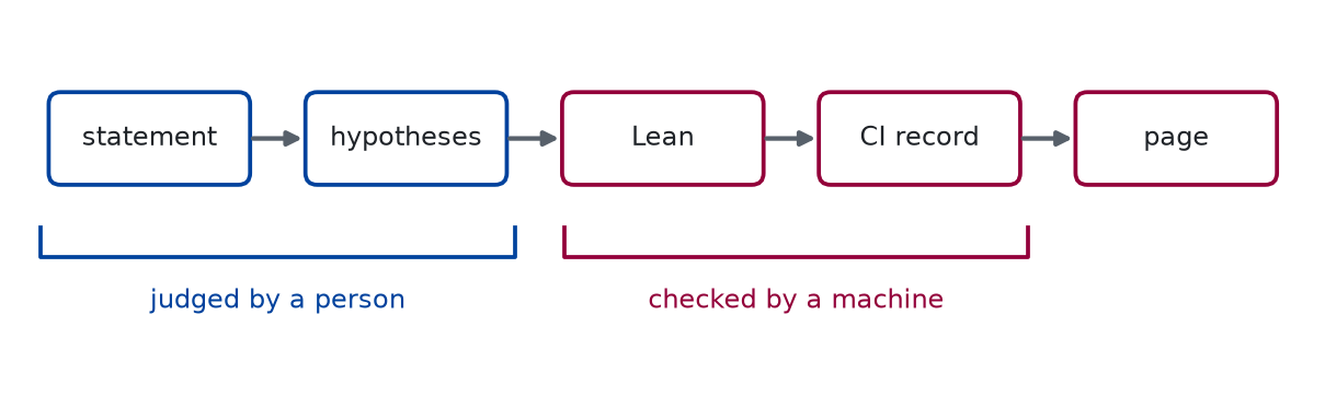
Between a statement on paper and a theorem on this page there are five steps, and the lesson depends on each:

def draw_theorem_pipeline() -> Figure:
    """From a statement to the page, as a sketch."""
    fig, ax = diagrams.canvas(6.4, 2.6, (-0.2, 12.8), (-1.2, 2.4))
    steps = ("statement", "hypotheses", "Lean", "CI record", "page")
    for i, name in enumerate(steps):
        x = 1.1 + 2.6 * i
        diagrams.state_box(
            ax, (x, 1.2), name, width=2.0, height=0.9, colour=0 if i < 2 else 1
        )
        if i:
            diagrams.arrow(ax, (x - 2.6 + 1.05, 1.2), (x - 1.05, 1.2), colour="#57606a")
    diagrams.line(ax, [(0.0, 0.3), (0.0, 0.0), (4.8, 0.0), (4.8, 0.3)], colour=0)
    diagrams.text(ax, (2.4, -0.45), "judged by a person", colour=0)
    diagrams.line(ax, [(5.3, 0.3), (5.3, 0.0), (10.0, 0.0), (10.0, 0.3)], colour=1)
    diagrams.text(ax, (7.65, -0.45), "checked by a machine", colour=1)
    fig.tight_layout()
    return fig

src/pbc/mechanics/experiments/proving_what_the_simulation_showed.py, lines 44 to 60, read from the repository when this page was built.

A row of five boxes joined by arrows: statement, hypotheses, Lean, CI record, page. A bracket under the statement and hypotheses boxes is labelled judged by a person. A bracket under the Lean and CI record boxes is labelled checked by a machine. — Figure 1: conceptual From a statement to a page. The hypotheses are part of the statement and are written out, not assumed. Lean accepts the file only if the proof builds, CI records the commit and the versions that built it, and the page reads its listings from that file. The machine checks the proof and the build record; the page is generated from that file and checked by the site build. Whether the statement is the right one to prove is a judgement of the author and the reader.

The diagram is a sketch of the process, and nothing in it is computed. It answers a question the section raises: if the compiler checks the proof, what is left for the reader to check? The statement and its hypotheses. A true theorem of a model that does not describe the oscillator proves nothing about the oscillator, and the assumptions list above is there so that this judgement can be made.

Constant acceleration

The first theorem. Its two hypotheses are the position and the velocity of the motion; its conclusion is the identity. The proof is two tactics.

/-- **Torricelli's identity.** A particle with constant acceleration `a`,
starting at `x₀` with velocity `v₀`, has at every time `t` the position `x`
and the velocity `v` of the two hypotheses `hx` and `hv`. Then
`v² = v₀² + 2 a (x - x₀)`: the speed is fixed by the distance covered,
whatever the time it took. -/
theorem velocity_sq_of_constant_acceleration
    (x₀ v₀ a t x v : ℝ)
    (hx : x = x₀ + v₀ * t + a * t ^ 2 / 2)
    (hv : v = v₀ + a * t) :
    v ^ 2 = v₀ ^ 2 + 2 * a * (x - x₀) := by
  subst hx hv
  ring

lean/PhysicsByConstruction/Mechanics/Kinematics.lean, lines 21 to 32, read from the repository when this page was built.

The mean-velocity form is proved the same way:

/-- The distance covered with constant acceleration equals the mean of the
initial and the final velocity times the time. -/
theorem displacement_of_mean_velocity
    (x₀ v₀ a t x v : ℝ)
    (hx : x = x₀ + v₀ * t + a * t ^ 2 / 2)
    (hv : v = v₀ + a * t) :
    x - x₀ = (v₀ + v) / 2 * t := by
  subst hx hv
  ring

lean/PhysicsByConstruction/Mechanics/Kinematics.lean, lines 36 to 44, read from the repository when this page was built.

The energy of the oscillator

The definition the theorems are about. noncomputable is Lean’s word for a definition on the real numbers, which cannot be evaluated by the compiler; it does not mean that the definition is vague.

/-- The mechanical energy of mass `m` on a spring `k`, at position `x` with
velocity `v`: kinetic `m v² / 2` plus potential `k x² / 2`. -/
noncomputable def springEnergy (m k x v : ℝ) : ℝ :=
  m * v ^ 2 / 2 + k * x ^ 2 / 2

lean/PhysicsByConstruction/Mechanics/EulerOscillator.lean, lines 23 to 26, read from the repository when this page was built.

One step multiplies the energy by the factor. The hypothesis hnewton is Newton’s law for the spring, hx' and hv' are the update rule, and the proof solves the law for the acceleration, substitutes the rule, and lets field_simp and ring check the identity.

/-- **One explicit Euler step multiplies the energy by `1 + (k / m) Δt²`.**

The state `(x, v)` is advanced to `(x', v')` by the rule of explicit Euler,
`hx'` and `hv'`, in which the acceleration `a` is the one at the old state.
`hnewton` is Newton's second law with the force of the spring, `m a = -k x`. -/
theorem euler_energy_step
    (m k x v a dt x' v' : ℝ) (hm : 0 < m)
    (hnewton : m * a = -k * x)
    (hx' : x' = x + dt * v)
    (hv' : v' = v + dt * a) :
    springEnergy m k x' v' = (1 + k / m * dt ^ 2) * springEnergy m k x v := by
  have ha : a = -k * x / m := by
    field_simp
    linarith [mul_comm m a]
  subst hx' hv' ha
  unfold springEnergy
  field_simp
  ring

lean/PhysicsByConstruction/Mechanics/EulerOscillator.lean, lines 30 to 47, read from the repository when this page was built.

The energy grows. This one is not an identity but an inequality, and it needs three more hypotheses: a positive spring constant, a step of non-zero size, and a positive energy before the step.

/-- **The energy never decreases, and grows when anything moves.** With a
positive mass and spring constant, a step of non-zero size multiplies a
positive energy by a factor greater than one. -/
theorem euler_energy_grows
    (m k x v a dt x' v' : ℝ) (hm : 0 < m) (hk : 0 < k)
    (hnewton : m * a = -k * x)
    (hx' : x' = x + dt * v)
    (hv' : v' = v + dt * a)
    (hdt : dt ≠ 0) (hE : 0 < springEnergy m k x v) :
    springEnergy m k x v < springEnergy m k x' v' := by
  rw [euler_energy_step m k x v a dt x' v' hm hnewton hx' hv']
  have : 0 < k / m * dt ^ 2 := by positivity
  nlinarith

lean/PhysicsByConstruction/Mechanics/EulerOscillator.lean, lines 51 to 63, read from the repository when this page was built.

And over any number of steps. The sequences x, v, and a stand for the whole run, and each hypothesis now holds for every step n.

/-- **After `n` steps the energy has been multiplied by `(1 + (k / m) Δt²)ⁿ`.**

`x` and `v` are the positions and velocities after each step, `a` the
accelerations at those states. The hypotheses say that every step is an
explicit Euler step of the spring. -/
theorem euler_energy_after_steps
    (m k dt : ℝ) (hm : 0 < m) (x v a : ℕ → ℝ)
    (hnewton : ∀ n, m * a n = -k * x n)
    (hx : ∀ n, x (n + 1) = x n + dt * v n)
    (hv : ∀ n, v (n + 1) = v n + dt * a n) (n : ℕ) :
    springEnergy m k (x n) (v n) =
      (1 + k / m * dt ^ 2) ^ n * springEnergy m k (x 0) (v 0) := by
  induction n with
  | zero => simp
  | succ n ih =>
    rw [euler_energy_step m k (x n) (v n) (a n) dt _ _ hm (hnewton n) (hx n) (hv n),
      ih, pow_succ]
    ring

lean/PhysicsByConstruction/Mechanics/EulerOscillator.lean, lines 67 to 84, read from the repository when this page was built.

Worked examples

Each theorem is a statement about all real numbers. The simulation can only sample it, and a sample is the right place to see which number the theorem is about. Everything in this section is numerical evidence: it is computed by the build, for the cases shown, in doubles.

The identity on the exact motion

The kinematics lesson’s function for the exact motion under constant acceleration is the pair of formulas of the hypotheses. The cell evaluates $v^2 - v_0^2 - 2a(x - x_0)$ along it, which the theorem says is zero. A value at the level of round-off is shown as a bound, because another machine would print other digits there.

FLOOR = 1e-12  # m^2/s^2, far above the round-off of this arithmetic
a = -9.81  # m/s^2
start = kinematics.State(t=0.0, x=0.0, v=20.0)
times = np.linspace(0.0, 4.0, 9)

src/pbc/mechanics/experiments/proving_what_the_simulation_showed.py, lines 26 to 29, read from the repository when this page was built.

def shown(value):
    """A residual as a number, or as the bound it is below."""
    return f"{value:.1e}" if abs(value) > FLOOR else f"below {FLOOR:.0e}"

src/pbc/mechanics/experiments/proving_what_the_simulation_showed.py, lines 63 to 65, read from the repository when this page was built.

def exact_residual(experiment: Experiment):
    """The residual of Torricelli's identity along the exact motion; record
    the table."""
    exact = kinematics.constant_acceleration(start, a, times)

    residual = exact.v**2 - start.v**2 - 2 * a * (exact.x - start.x)
    experiment.table(
        "exact-residual",
        [
            (t, x, v, shown(r))
            for t, x, v, r in zip(times, exact.x, exact.v, residual, strict=True)
        ],
        [
            ("t", "s", ".2f"),
            ("x", "m", ".2f"),
            ("v", "m/s", ".2f"),
            ("v^2 - v0^2 - 2 a (x - x0)", "m^2/s^2", ""),
        ],
        "The residual of Torricelli's identity along the exact motion of a throw "
        "upward at 20 m/s.",
    )
    return residual

src/pbc/mechanics/experiments/proving_what_the_simulation_showed.py, lines 68 to 89, read from the repository when this page was built.

The residual of Torricelli's identity along the exact motion of a throw upward at 20 m/s.
t (s)	x (m)	v (m/s)	v^2 - v0^2 - 2 a (x - x0) (m^2/s^2)
0.00	0.00	20.00	below 1e-12
0.50	8.77	15.09	below 1e-12
1.00	15.09	10.19	below 1e-12
1.50	18.96	5.29	below 1e-12
2.00	20.38	0.38	below 1e-12
2.50	19.34	-4.53	below 1e-12
3.00	15.85	-9.43	below 1e-12
3.50	9.91	-14.34	below 1e-12
4.00	1.52	-19.24	below 1e-12

Numerically verified (one throw, nine instants, doubles): Along the exact motion the residual of the identity is zero to round-off. Its largest absolute value in the table is below 1e-12 $\mathrm{m}^2/\mathrm{s}^2$ , and the first row is zero identically, as the theorem predicts for $t = 0$ . The numbers are not the proof: they are the same statement, seen on a few of the infinitely many instants that the theorem covers.

What the hypotheses are worth

The identity needs the formula for the position. A simulation does not satisfy it, and the theorem does not say it should. Explicit Euler, run on the same fall, has the exact velocity and a position that lags behind the formula, and the residual of the identity on the simulated motion is not zero. It is exactly $a^2\,t\,\Delta t$ : the quantity the identity measures is the error of the method. This follows from the update rule in four lines.

Explicit Euler moves by the old velocity, and its velocity is exact because the acceleration is constant: at step $k$ it is $v_k = v_0 + a\,k\,\Delta t$ . After $n$ steps, with $t = n\,\Delta t$ ,

$x_n - x_0 = \sum_{k=0}^{n-1} v_k\,\Delta t = n\,v_0\,\Delta t + a\,\Delta t^2\,\frac{n(n-1)}{2} = v_0\,t + \tfrac12\,a\,t^2 - \tfrac12\,a\,t\,\Delta t.$

The position is the exact one minus $\tfrac12\,a\,t\,\Delta t$ . Put it into the identity with the exact velocity $v = v_0 + a\,t$ : the left side $v^2 - v_0^2$ is $2 v_0 a t + a^2 t^2$ , twice the acceleration times the distance is $2 v_0 a t + a^2 t^2 - a^2 t \Delta t$ , and the difference is

$v^2 - v_0^2 - 2a\,(x_n - x_0) = a^2\,t\,\Delta t.$

The cell checks the derivation against the simulation.

def euler_residual(experiment: Experiment):
    """The residual of the identity on the explicit Euler fall against the
    derivation; record the table."""
    fall_dt = 0.25  # s
    fall = kinematics.simulate(start, lambda t: a, fall_dt, 16)
    residual = fall.v**2 - start.v**2 - 2 * a * (fall.x - start.x)
    predicted = a**2 * fall.t * fall_dt

    experiment.table(
        "euler-residual",
        list(zip(fall.t, residual, predicted, strict=True))[::4],
        [
            ("t", "s", ".2f"),
            ("residual on the simulated motion", "m^2/s^2", ".3f"),
            ("a^2 t dt", "m^2/s^2", ".3f"),
        ],
        "The residual of the identity on the explicit Euler fall, and the value the "
        "derivation gives, to three decimals.",
    )
    return len(fall.t), np.max(np.abs(residual - predicted))

src/pbc/mechanics/experiments/proving_what_the_simulation_showed.py, lines 92 to 111, read from the repository when this page was built.

The residual of the identity on the explicit Euler fall, and the value the derivation gives, to three decimals.
t (s)	residual on the simulated motion (m^2/s^2)	a^2 t dt (m^2/s^2)
0.00	0.000	0.000
1.00	24.059	24.059
2.00	48.118	48.118
3.00	72.177	72.177
4.00	96.236	96.236

Numerically verified (constant acceleration, explicit Euler, any step; derived above and recomputed here for one step size): On the explicit Euler fall under constant acceleration, the residual of the identity is $a^2\,t\,\Delta t$ . The two columns agree at every step of the run: the largest difference over all 17 instants is below 1e-12 $\mathrm{m}^2/\mathrm{s}^2$ .

A theorem has the hypotheses it states and not the ones that are convenient. Here the position formula is a hypothesis the simulation does not meet, so the conclusion does not follow for it, and the residual is a property of the simulated motion that the theorem does not describe.

The factor, step after step

The harmonic oscillator of the earlier lesson: 0.5 kg on a spring of 2 N/m, pulled out one metre. The cell runs explicit Euler for three periods and compares the measured energy after $n$ steps with the conclusion of euler_energy_after_steps, $(1 + k\,\Delta t^2/m)^n E_0$ .

mass = 0.5  # kg
k = 2.0  # N/m
period = 2 * np.pi / angular_frequency(mass, k)
released = State(t=0.0, x=1.0, v=0.0)
oscillator = newton(mass, spring(k))

steps_per_period = 64
n_steps = 3 * steps_per_period
dt = period / steps_per_period

src/pbc/mechanics/experiments/proving_what_the_simulation_showed.py, lines 32 to 40, read from the repository when this page was built.

def energy_factor(experiment: Experiment):
    """The energy of the oscillator after whole periods against the theorem;
    record the table."""
    simulated = simulate(released, oscillator, dt, n_steps)
    measured = energy(simulated, mass, k)
    factor = 1 + k / mass * dt**2
    proved = factor ** np.arange(n_steps + 1) * measured[0]

    relative = np.abs(measured / proved - 1)
    rows = [
        (n, measured[n], proved[n]) for n in range(0, n_steps + 1, steps_per_period)
    ]
    experiment.table(
        "energy-factor",
        rows,
        [
            ("steps", "", "d"),
            ("energy measured", "J", ".4f"),
            ("energy from the theorem", "J", ".4f"),
        ],
        "The energy of the simulated oscillator after whole periods, and the energy "
        "the theorem predicts, to four decimals.",
    )
    return factor, relative

src/pbc/mechanics/experiments/proving_what_the_simulation_showed.py, lines 114 to 137, read from the repository when this page was built.

The energy of the simulated oscillator after whole periods, and the energy the theorem predicts, to four decimals.
steps	energy measured (J)	energy from the theorem (J)
0	1.0000	1.0000
64	1.8476	1.8476
128	3.4137	3.4137
192	6.3072	6.3072

The factor per step is 1.009638. The measured energy and the predicted one agree at every step of the run, not only in the rows shown: the largest relative difference is below 1e-12.

Numerically verified (one oscillator, one step size, doubles): The energy of the simulated oscillator follows the factor of the theorem at every step.

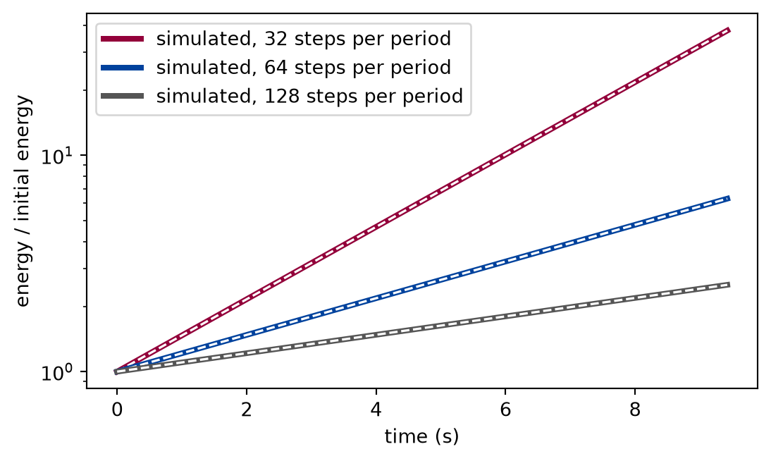
def draw_proved_energy_growth() -> Figure:
    """The simulated energy and the theorem at three steps."""
    fig, ax = plt.subplots(figsize=(6.4, 3.6))
    for n, colour in ((32, "#93003a"), (64, "#00429d"), (128, "#555555")):
        step = period / n
        steps = 3 * n
        simulated = energy(simulate(released, oscillator, step, steps), mass, k)
        theorem = (1 + k / mass * step**2) ** np.arange(steps + 1) * simulated[0]
        time = step * np.arange(steps + 1)
        ax.semilogy(
            time,
            simulated / simulated[0],
            color=colour,
            linestyle="-",
            linewidth=3,
            label=f"simulated, {n} steps per period",
        )
        ax.semilogy(
            time,
            theorem / simulated[0],
            color="white",
            linestyle="--",
            linewidth=1.2,
            label="_nolegend_",
        )
    ax.set_xlabel("time (s)")
    ax.set_ylabel("energy / initial energy")
    ax.legend(loc="upper left")
    return fig

src/pbc/mechanics/experiments/proving_what_the_simulation_showed.py, lines 140 to 168, read from the repository when this page was built.

Plot of the energy divided by the initial energy against time in seconds, with a logarithmic vertical axis. Three solid curves rise from the same point at time zero, one for each of three time steps; the coarsest rises steepest. Over each solid curve lies a dashed curve of the prediction of the theorem, so that the two cannot be told apart. — Figure 2: simulated The simulated energy (solid) and the energy the theorem predicts (dashed) lie on each other for three time steps; the coarser the step, the faster the energy grows.

The simulated curves lie on the predicted ones, which were computed from the factor alone and checked here against runs. What the figure cannot show is why: the theorem is the reason, and it is the same reason for every step size, not only for the three drawn.

What the proofs do not cover

The Python code. Nothing here is a statement about pbc.mechanics. The theorems are about a model of explicit Euler written in Lean; that the Python code implements that model is what the unit tests and the examples above check, to round-off, for the cases they run. Proving a program correct is a different and much larger project, and this site does not claim it.
Floating-point arithmetic. ℝ is exact. A double carries a relative error of about $10^{-16}$ per operation, and no theorem on this page speaks about it.
Continuous time. The position and velocity formulas are hypotheses. That they solve the equations of motion is a statement about derivatives, and it is not proved here.
Other methods. The factor belongs to explicit Euler. The other steppers of the mechanics course, introduced in its numerical integrators lesson (symplectic Euler, velocity Verlet, and the classical Runge-Kutta method), satisfy other relations; the second exercise defines one of them in full and shows that the theorem does not describe it.
That the model is physics. A Lean proof tells us what follows from the hypotheses. Whether a real spring obeys $m\,a = -k\,x$ is settled by measuring it. No theorem of this lesson is a claim about a measurement, and the label of each one states the model it is about.
The examples. The tables are numerical evidence for the cases run, in doubles. They illustrate the theorems; they do not add to them.

Self-check. Suppose the Python function that steps the oscillator had a bug, so that its energy after a step were $1.0001$ times what the theorem says. Would the theorem euler_energy_step become false? What would the table of the worked example show, and what does that tell you about what the proof covers?

With scripts, you can record in this browser that you answered this question.

Solution to the self-check

The theorem would stay true, because it is about the rule written in Lean on the real numbers, not about the Python function. The table would show it: the measured energy would stop agreeing with the energy predicted from the factor, by far more than round-off. The proof says what an explicit Euler step does in the model; the table checks that the program is a step of that model, for the cases it runs. Each is evidence for a different statement, and neither replaces the other.

Exercises

Exercise 1. Which hypotheses can go? In euler_energy_step, the hypothesis hm : 0 < m is used. What happens to the theorem without it, if the mass is zero? And in euler_energy_grows, which of the hypotheses hk, hdt, and hE can be dropped if the conclusion is changed from “strictly greater” to “at least”?

Solution to exercise 1

With $m = 0$ the hypothesis hnewton reads $0 = -k\,x$ , which constrains the position and says nothing about $a$ , so the acceleration cannot be recovered and the step is not determined by the law of motion. The proof divides by $m$ ; the statement needs the hypothesis for that, and the physics needs it because a particle of zero mass has no inertia.

For the weaker conclusion, the factor $1 + (k/m)\,\Delta t^2$ is at least one whenever $k \ge 0$ , so hk can become 0 ≤ k, hdt is no longer needed because $\Delta t^2 \ge 0$ for every real step, and hE becomes 0 ≤ springEnergy m k x v. What is lost is exactly what the strict inequality says: the energy grows only if there is energy and something moves.

Exercise 2. A rule the theorem does not describe. Symplectic Euler updates the velocity first and then moves the particle with the new velocity: $v' = v + \Delta t\,a$ , $x' = x + \Delta t\,v'$ . Which hypothesis of euler_energy_step does this violate? Compute the ratio of the energies after and before a step for the oscillator of the examples, and see whether it is constant.

Solution to exercise 2

The hypothesis hx' : x' = x + dt * v fails: the new position uses v', not v. The theorem says nothing about the rule, and the ratio is not constant, as the cell shows: it depends on the state.

def symplectic_step(x, v):
    v_new = v - k / mass * x * dt
    return x + dt * v_new, v_new

src/pbc/mechanics/experiments/proving_what_the_simulation_showed.py, lines 171 to 173, read from the repository when this page was built.

def spring_energy(x, v):
    return 0.5 * mass * v**2 + 0.5 * k * x**2

src/pbc/mechanics/experiments/proving_what_the_simulation_showed.py, lines 176 to 177, read from the repository when this page was built.

def symplectic_ratios(experiment: Experiment, factor) -> None:
    """Exercise: the ratio of the energies after and before a step for
    symplectic Euler over one period, and for explicit Euler; record the
    table."""
    x, v = 1.0, 0.0
    ratios = []
    for _ in range(steps_per_period):
        x_new, v_new = symplectic_step(x, v)
        ratios.append(spring_energy(x_new, v_new) / spring_energy(x, v))
        x, v = x_new, v_new

    experiment.table(
        "symplectic-ratios",
        [
            ("symplectic Euler, smallest over one period", min(ratios)),
            ("symplectic Euler, largest over one period", max(ratios)),
            ("explicit Euler, at every step", factor),
        ],
        [("rule", "", ""), ("energy after a step / energy before", "", ".4f")],
        "The ratio of the energies after and before a step for the two rules, to "
        "four decimals.",
    )

src/pbc/mechanics/experiments/proving_what_the_simulation_showed.py, lines 180 to 201, read from the repository when this page was built.

The ratio of the energies after and before a step for the two rules, to four decimals.
rule	energy after a step / energy before
symplectic Euler, smallest over one period	0.9904
symplectic Euler, largest over one period	1.0097
explicit Euler, at every step	1.0096

The ratio swings above and below one, so the energy of this rule oscillates instead of growing, and a different theorem, with a different invariant, describes it.

Exercise 3. The error of Euler on a fall, as a theorem. The second worked example derived the residual $a^2\,t\,\Delta t$ of the identity on the simulated fall. Write the statement of a Lean theorem that says it, and say which hypothesis of velocity_sq_of_constant_acceleration you change and how the proof changes.

Solution to exercise 3

The only hypothesis that changes is hx, which becomes the position of explicit Euler after $n$ steps, with $t = n\,\Delta t$ in place of a free time. The theorem is a statement about the same real numbers with a new conclusion. It is a sketch, not part of the project, so it carries the marker:

Not verified. The build of this site did not run or check the material in this box.

theorem euler_fall_residual (x₀ v₀ a dt t x v : ℝ)
    (hx : x = x₀ + v₀ * t + a * t ^ 2 / 2 - a * t * dt / 2)
    (hv : v = v₀ + a * t) :
    v ^ 2 - v₀ ^ 2 - 2 * a * (x - x₀) = a ^ 2 * t * dt := by
  subst hx hv
  ring

The proof is again subst and ring: the polynomial identity of the derivation, with a different right-hand side. What a theorem like this would not say is that the sum over steps gives that position; that is an induction on the number of steps, as in euler_energy_after_steps.

Check this proof

This page was built from commit 6417e2ff90258bd2d2ba21d217eb7666fd24f680 of the repository.

In a clone at that commit, with the pinned Lean toolchain, this command in lean/ checks the proofs of this page:

lake build PhysicsByConstruction.Mechanics.Kinematics PhysicsByConstruction.Mechanics.EulerOscillator

Files, tests, and every command

The files behind it:

site/lessons/lean/01-proving-what-the-simulation-showed/index.qmd: this page, with every code cell.
lean/PhysicsByConstruction/Mechanics/Kinematics.lean: a Lean file the page shows.
lean/PhysicsByConstruction/Mechanics/EulerOscillator.lean: a Lean file the page shows.
src/pbc/mechanics/kinematics.py: code the experiment runs.
src/pbc/mechanics/oscillator.py: code the experiment runs.
src/pbc/mechanics/experiments/proving_what_the_simulation_showed.py: code the experiment runs.
src/pbc/experiment.py: code the experiment runs.
tests/unit/test_kinematics.py: tests of that code.
tests/unit/test_oscillator.py: tests of that code.
tests/unit/test_proving_what_the_simulation_showed_experiment.py: tests of that code.

With Git and uv, and elan for the proofs, installed (see the setup page), run:

git clone https://github.com/taspinar/physics-by-construction.git
cd physics-by-construction
git checkout 6417e2ff90258bd2d2ba21d217eb7666fd24f680
uv sync --locked --no-dev
uv run --locked --no-dev python -m pbc.mechanics.experiments.proving_what_the_simulation_showed results
cd lean
lake exe cache get
lake build PhysicsByConstruction.Mechanics.Kinematics PhysicsByConstruction.Mechanics.EulerOscillator

The experiment writes every figure of this page into results/, as <label>.png, and every number and table of the page, as the page shows it, into results/results.json. Its numbers match this page to the digits shown, and its figure files are the ones the page shows; digits beyond those can differ between machines, because floating-point libraries differ. Change the code of the experiment and run it again to see what changes.

lake build compiles the proofs of this page with the Lean toolchain that elan installs; the first run fetches the Mathlib build cache, which is large. The setup page says how to install elan.