Induction: magnetic flux and the electromotive force

The voltage induced around a loop computed as the work per charge along the wire, and the magnetic flux through it computed as a surface integral, apart: for a loop moving through a non-uniform field, a turning coil, and a loop at rest beside a changing field, the voltage is minus the rate of change of the flux.

Course

Electromagnetism, lesson 3 of 3

Slot

EM3, Faraday’s law and induction

Methods

Simulation

Difficulty

Intermediate, level 2 of 3

What you’ll learn

Compute the magnetic flux through a loop as a surface integral and its rate of change by a central difference
Compute the electromotive force around a loop as the line integral of the force per charge on the charges of the wire
Check Faraday’s law for a moving loop, a turning coil, and a loop at rest in a changing field
Explain why a loop can have an induced voltage where the magnetic field on the wire is nearly zero, and none where the electric field is not

Prerequisites

Electric fields, superposition, and the potential, Charged particles in electric and magnetic fields.

Before you begin

Vectors: the cross product in three dimensions
Calculus: line integrals and integrals over a surface

Related

none

Previous

Charged particles in electric and magnetic fields

Next

An agent runs an experiment

With scripts, this page keeps a record in your browser of whether you completed the lesson. Nothing is stored without them.

With scripts, this place suggests what to do next, with the reason, from the progress saved in your browser. Without them, follow the learning path.

Move a magnet in and out of a coil of wire and a current flows in the wire, though no battery is connected. A bicycle dynamo lights its lamp the same way, and so does every generator of a power station: a coil turns in a magnetic field, and a voltage appears between its ends. A transformer does it with nothing moving at all, by changing the field through a coil.

Faraday found the rule that covers all of these: the voltage around a loop, its electromotive force, is minus the rate at which the magnetic flux through the loop changes. This lesson does not assume the rule. It computes the voltage from the force on the charges in the wire, the Lorentz force of the previous lesson and the induced electric field, integrated around the loop. It computes the flux, separately, by integrating the field over the surface the loop bounds, and differentiates it in time. Then it asks whether the two agree, for a loop that slides through a field that is not uniform, for a coil that turns, and for a loop at rest beside a field that grows. The surprises are in the last case: a loop can have a voltage where the field on its wire is nearly zero, and none where the electric field on it is strong.

Assumptions

Thin wire, flat loops. The loop is a curve without thickness, the edge of a flat rectangle. A real coil has a thickness and many turns; for a coil of several turns the voltage is the sum over the turns.
No current, or a current too small to matter. The voltage is computed for an open loop, or one with a very large resistance. A current in the loop would make a field of its own that opposes the change, which is the content of Lenz’s rule, and changes the flux.
Slow compared with light. The wire moves far slower than light, and the fields change slowly enough that the time light takes to cross the loop does not matter. Then the force per charge on a charge moving with the wire is $\mathbf{E} + \mathbf{u}\times\mathbf{B}$ , with $\mathbf{u}$ the velocity of the wire there.
Given fields. The magnetic and the induced electric field are given in closed form, not computed from currents. The flux tube of the third example is a model of the field inside and near a long coil, with smooth edges so that its integrals are accurate.
Quadrature and a difference. The integrals are Gauss-Legendre rules, accurate for smooth fields; the rate of change of the flux is a central difference, whose error falls as the square of its step.

Faraday’s law

The electromotive force and the flux

A charge carried along by the wire at the velocity $\mathbf{u}$ feels the force $q(\mathbf{E} + \mathbf{u}\times\mathbf{B})$ . The electromotive force of the loop is the work this force does per unit charge on one trip around it,

$\mathcal{E} = \oint \left(\mathbf{E} + \mathbf{u}\times\mathbf{B}\right)\cdot \mathrm{d}\boldsymbol{\ell},$

and it is the voltage a meter would read across a small gap in the loop. The flux is the integral of the magnetic field over the surface that the loop bounds, with the normal $\hat{\mathbf{n}}$ that the sense of the loop picks by the right-hand rule:

$\Phi = \int_S \mathbf{B}\cdot\hat{\mathbf{n}}\,\mathrm{d}A .$

Faraday’s law, in the form called the flux rule, says

$\mathcal{E} = -\frac{\mathrm{d}\Phi}{\mathrm{d}t}.$

Why it holds: two ways for the flux to change

The flux through a loop changes for two reasons, and each corresponds to one of the two terms of the force.

The loop moves. In a static field a moving loop sweeps out a strip with each piece $\mathrm{d}\boldsymbol{\ell}$ of its edge, of area $\mathbf{u}\,\mathrm{d}t\times\mathrm{d}\boldsymbol{\ell}$ per time $\mathrm{d}t$ . A magnetic field has no sources, $\nabla\cdot\mathbf{B} = 0$ , so the flux that the loop gains is the flux through those strips,

$\begin{aligned} \frac{\mathrm{d}\Phi}{\mathrm{d}t} &= \oint \mathbf{B}\cdot(\mathbf{u}\times\mathrm{d}\boldsymbol{\ell}) \\ &= -\oint (\mathbf{u}\times\mathbf{B})\cdot\mathrm{d}\boldsymbol{\ell}, \end{aligned}$

the motional term. For a rectangle of height $h$ moving at $v$ along $x$ through a field $B_z(x)$ , only the two sides across the motion count, and $\mathcal{E} = -v\,h\,(B_z(x_{\text{front}}) - B_z(x_{\text{back}}))$ .

The field changes. A magnetic field that changes in time comes with an electric field that circulates around it: the Maxwell-Faraday equation $\nabla\times\mathbf{E} = -\partial\mathbf{B}/\partial t$ , which by Stokes’s theorem gives $\oint\mathbf{E}\cdot\mathrm{d}\boldsymbol{\ell} = -\int_S \partial\mathbf{B}/\partial t\cdot\hat{\mathbf{n}}\,\mathrm{d}A$ for a loop at rest. In terms of the potentials, $\mathbf{B} = \nabla\times\mathbf{A}$ and the induced field is $\mathbf{E} = -\partial\mathbf{A}/\partial t$ .

Neither statement is used to compute anything below. The program integrates the force along the wire and the field over the surface with separate rules, and differentiates the flux numerically; the law is what the comparison tests.

The flux tube

The third example uses a tube of field along $z$ , strongest on its axis and falling off with the distance $r$ from it over a width $a$ , $B_z = B_0\,e^{-r^2/a^2}$ , a smooth model of the field inside a long coil. Its vector potential points around the axis,

$A_\varphi(r) = \frac{B_0\,a^2}{2r}\left(1 - e^{-r^2/a^2}\right),$

and gives the field by $B_z = \frac{1}{r}\frac{\partial (r A_\varphi)}{\partial r}$ . When $B_0$ grows at the rate $\dot B_0$ , the induced electric field is $E_\varphi = -\partial A_\varphi/\partial t$ , the same expression with $\dot B_0$ in place of $B_0$ and a minus sign. Outside the tube the magnetic field is nearly zero, yet the electric field falls only as $1/r$ : a loop far from the tube still sits in an induced field.

Code

The loop is a Rectangle; flux integrates the field over it, and emf integrates the force per charge around its edge. The two do not call each other. flux_rate is the central difference of the flux in time.

def emf(
    loop: Rectangle,
    *,
    electric: VectorField | None = None,
    magnetic: VectorField | None = None,
    velocity: VectorField | None = None,
    nodes: int = 24,
) -> float:
    """The EMF around ``loop`` in its sense, in V: the line integral of the
    force per unit charge E + u x B on a charge carried by the wire, where
    ``velocity`` gives the velocity u (m/s) of the wire at each of its
    points. A field that is not given is zero; a wire at rest feels only E.
    """
    points, elements = loop.edge(nodes)
    force = np.zeros_like(points)
    if electric is not None:
        force += electric(points)
    if magnetic is not None and velocity is not None:
        force += np.cross(velocity(points), magnetic(points))
    return float(np.sum(force * elements))

src/pbc/electromagnetism/induction.py, lines 103 to 122, read from the repository when this page was built.

def flux(magnetic: VectorField, loop: Rectangle, *, nodes: int = 24) -> float:
    """The flux of ``magnetic`` (a function of the points) through ``loop``
    along its normal, by Gauss-Legendre in both directions: in Wb."""
    points, weights = loop.surface(nodes)
    return float(np.sum(weights * (magnetic(points) @ loop.normal)))

src/pbc/electromagnetism/induction.py, lines 96 to 100, read from the repository when this page was built.

def flux_tube_fields(
    points: ArrayLike, *, strength: float, rate: float, width: float
) -> tuple[Array, Array]:
    """The induced electric field and the magnetic field (E, B) of a tube of
    flux along z: B = B0 exp(-r^2 / a^2) z, with B0 = ``strength`` (T)
    changing at ``rate`` (T/s) and a = ``width`` (m).

    Both come from the vector potential A = B0 a^2 (1 - exp(-r^2/a^2)) /
    (2 r) along phi: B = curl A, and the induced field E = -dA/dt, which
    is -rate a^2 (1 - exp(-r^2/a^2)) / (2 r) along phi. Neither uses
    Faraday's law.
    """
    points = np.asarray(points, dtype=float)
    x, y = points[..., 0], points[..., 1]
    r2 = x**2 + y**2
    profile = np.exp(-r2 / width**2)
    # (1 - exp(-r^2/a^2)) / r^2, which tends to 1/a^2 on the axis
    safe = np.where(r2 > 0.0, r2, 1.0)
    ratio = np.where(r2 > 0.0, -np.expm1(-r2 / width**2) / safe, 1.0 / width**2)
    # E_phi phi = E_phi / r (-y, x, 0)
    e_over_r = -0.5 * rate * width**2 * ratio
    electric = np.stack([-e_over_r * y, e_over_r * x, np.zeros_like(x)], axis=-1)
    magnetic = np.stack(
        [np.zeros_like(x), np.zeros_like(x), strength * profile], axis=-1
    )
    return electric, magnetic

src/pbc/electromagnetism/induction.py, lines 133 to 158, read from the repository when this page was built.

Worked examples

A uniform field is a function that gives the same vector at every point:

def uniform(vector):
    vector = np.asarray(vector, dtype=float)
    return lambda points: np.broadcast_to(vector, points.shape)

src/pbc/electromagnetism/experiments/faradays_law_and_induction.py, lines 33 to 35, read from the repository when this page was built.

A loop moving through a non-uniform field

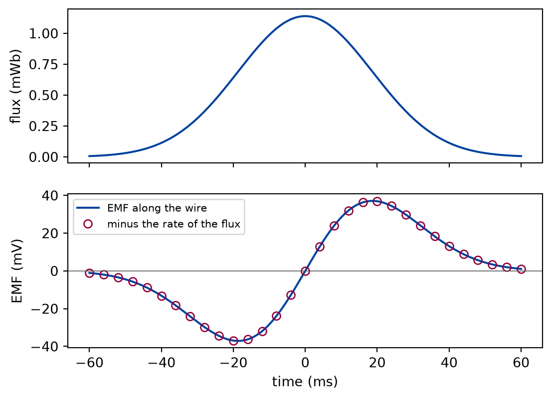
A field along $z$ has the profile of a bump in $x$ : 0.5 T at its peak, falling off over 5 cm. A rectangular loop of 4 cm along $x$ by 6 cm along $y$ moves through it at 2 m/s, centred on the peak at the time zero. The EMF is computed from $\mathbf{u}\times\mathbf{B}$ along the wire and compared with minus the rate of change of the flux, with a step of 10 μs, at times across the passage.

PEAK = 0.5  # T
BUMP = 0.05  # m
SPEED = 2.0  # m/s
WIDTH, HEIGHT = 0.04, 0.06  # m
STEP = 1e-5  # s, the step of the central difference
times = np.linspace(-0.06, 0.06, 241)  # s
FARADAY_TOLERANCE = 1e-6  # a chosen tolerance, relative to the largest EMF

src/pbc/electromagnetism/experiments/faradays_law_and_induction.py, lines 39 to 45, read from the repository when this page was built.

def bump(points):
    x = points[..., 0]
    return np.stack([0 * x, 0 * x, PEAK * np.exp(-((x / BUMP) ** 2))], axis=-1)

src/pbc/electromagnetism/experiments/faradays_law_and_induction.py, lines 49 to 51, read from the repository when this page was built.

def loop_at(t):
    return Rectangle(
        [SPEED * t - WIDTH / 2, -HEIGHT / 2, 0.0], [WIDTH, 0.0, 0.0], [0.0, HEIGHT, 0.0]
    )

src/pbc/electromagnetism/experiments/faradays_law_and_induction.py, lines 54 to 57, read from the repository when this page was built.

def moving_loop_run(experiment: Experiment) -> Passage:
    """The EMF of the moving loop from u x B along the wire against minus
    the rate of its flux; record the table of a few times."""
    carried = uniform([SPEED, 0.0, 0.0])
    fluxes = np.array([flux(bump, loop_at(t)) for t in times])
    motional = np.array(
        [emf(loop_at(t), magnetic=bump, velocity=carried) for t in times]
    )
    from_flux = np.array(
        [-flux_rate(lambda s: flux(bump, loop_at(s)), t, STEP) for t in times]
    )
    gap = float(np.max(np.abs(motional - from_flux)) / np.max(np.abs(motional)))
    assert gap < FARADAY_TOLERANCE, "the motional EMF is not -dPhi/dt"

    shown = [
        0,
        60,
        100,
        140,
        180,
        240,
    ]  # the time zero, where both are zero, is left out
    experiment.table(
        "moving-loop-run",
        [
            (times[i] * 1e3, fluxes[i] * 1e3, motional[i] * 1e3, from_flux[i] * 1e3)
            for i in shown
        ],
        [
            ("time", "ms", ".1f"),
            ("flux", "mWb", ".5f"),
            ("EMF along the wire", "mV", ".5f"),
            ("minus the rate of the flux", "mV", ".5f"),
        ],
        "The flux through the moving loop, its EMF from the force on the charges "
        "of the wire, and minus the rate of change of the flux, at a few of the "
        "computed times, to five decimals.",
    )
    return Passage(fluxes, motional, from_flux, gap)

src/pbc/electromagnetism/experiments/faradays_law_and_induction.py, lines 71 to 109, read from the repository when this page was built.

The flux through the moving loop, its EMF from the force on the charges of the wire, and minus the rate of change of the flux, at a few of the computed times, to five decimals.
time (ms)	flux (mWb)	EMF along the wire (mV)	minus the rate of the flux (mV)
-60.0	0.00612	-1.07532	-1.07532
-30.0	0.31139	-26.99926	-26.99926
-10.0	0.98650	-28.36245	-28.36245
10.0	0.98650	28.36245	28.36245
30.0	0.31139	26.99926	26.99926
60.0	0.00612	1.07532	1.07532

def draw_moving_loop(passage: Passage) -> Figure:
    """The flux through the passing loop, and its EMF computed both ways."""
    fig, (top, bottom) = plt.subplots(2, 1, figsize=(6.4, 4.6), sharex=True)
    top.plot(times * 1e3, passage.fluxes * 1e3, color=FIGURE_COLOURS[0])
    top.set_ylabel("flux (mWb)")
    bottom.plot(
        times * 1e3,
        passage.motional * 1e3,
        color=FIGURE_COLOURS[0],
        label="EMF along the wire",
    )
    bottom.plot(
        times[::8] * 1e3,
        passage.from_flux[::8] * 1e3,
        "o",
        markerfacecolor="none",
        color=FIGURE_COLOURS[1],
        label="minus the rate of the flux",
    )
    bottom.axhline(0.0, color=FIGURE_COLOURS[2], linewidth=0.6)
    bottom.set_xlabel("time (ms)")
    bottom.set_ylabel("EMF (mV)")
    bottom.legend(fontsize=8)
    return fig

src/pbc/electromagnetism/experiments/faradays_law_and_induction.py, lines 112 to 135, read from the repository when this page was built.

Two stacked plots against time. The upper one shows the flux as a single smooth hump centred at time zero. The lower one shows the EMF as a solid line that dips below zero before time zero, crosses zero at the peak of the flux, and rises above zero after it, antisymmetric about zero. Open circles for minus the rate of the flux lie on the line throughout. — Figure 1: simulated A loop passing through a bump of field. Top: the flux through it rises and falls. Bottom: the EMF from the force on the charges of the wire (line) and minus the rate of change of the flux (markers) are one curve, negative while the flux grows and positive while it falls.

Numerically verified (a rigid rectangular loop translated through a static field, a central difference of the stated step): The EMF of a loop moving through a static, non-uniform magnetic field, computed from the force $\mathbf{u}\times\mathbf{B}$ on the charges of the wire, equals minus the rate of change of the flux through the loop. At every one of the 241 times the two agree to 1.1e-07 of the largest EMF, inside the chosen tolerance of 1e-06; what remains is the error of the central difference. The sign is Lenz’s: while the loop enters the field and its flux grows, the EMF is negative, in the sense that would drive a current whose own field opposes the growth. At the time zero the loop is centred on the peak, the flux is largest, and the two sides across the motion sit in equal fields, so the EMF is zero. The data are simulated, and the check is the flux rule.

A coil turning in a uniform field

A coil of 10 cm by 20 cm turns at 50 Hz about its long axis in a uniform field of 0.3 T across the axis: a generator of a single turn. Each point of the wire moves with the velocity $\boldsymbol{\omega}\times\mathbf{r}$ . The EMF from the force along the wire is compared over one turn with minus the rate of the flux and with $B A \omega \sin\omega t$ .

FIELD = np.array([0.3, 0.0, 0.0])  # T
OMEGA = 2 * np.pi * 50.0  # rad/s
COIL = dict(angular_velocity=OMEGA, width=0.1, height=0.2)
turn_times = np.linspace(0.0, 0.02, 81)  # s, one turn

src/pbc/electromagnetism/experiments/faradays_law_and_induction.py, lines 139 to 142, read from the repository when this page was built.

def coil_run(experiment: Experiment) -> tuple[float, float]:
    """The EMF of the turning coil along the wire against minus the rate of
    its flux and against B A omega sin(omega t); record the table, return
    the largest gap and the peak."""
    area = COIL["width"] * COIL["height"]
    spin = np.array([0.0, 0.0, OMEGA])

    def turning(points):
        return np.cross(spin, points)

    coil_emf = np.array(
        [
            emf(rotating_coil(t, **COIL), magnetic=uniform(FIELD), velocity=turning)
            for t in turn_times
        ]
    )
    coil_from_flux = np.array(
        [
            -flux_rate(
                lambda s: flux(uniform(FIELD), rotating_coil(s, **COIL)), t, 1e-7
            )
            for t in turn_times
        ]
    )
    generator = FIELD[0] * area * OMEGA * np.sin(OMEGA * turn_times)
    peak = FIELD[0] * area * OMEGA
    coil_gap = float(np.max(np.abs(coil_emf - coil_from_flux)) / peak)
    formula_gap = float(np.max(np.abs(coil_emf - generator)) / peak)
    gap = max(coil_gap, formula_gap)
    assert gap < FARADAY_TOLERANCE, "the coil is not a generator"

    experiment.table(
        "coil-run",
        [
            ("EMF along the wire", np.max(coil_emf), np.min(coil_emf)),
            (
                "minus the rate of the flux",
                np.max(coil_from_flux),
                np.min(coil_from_flux),
            ),
            ("B A ω sin ωt", peak, -peak),
        ],
        [("computed as", "", ""), ("largest", "V", ".5f"), ("smallest", "V", ".5f")],
        "The largest and smallest EMF of the turning coil over one turn, from the "
        "force along the wire, from the rate of the flux, and from the generator "
        "formula, to five decimals.",
    )
    return gap, peak

src/pbc/electromagnetism/experiments/faradays_law_and_induction.py, lines 146 to 193, read from the repository when this page was built.

The largest and smallest EMF of the turning coil over one turn, from the force along the wire, from the rate of the flux, and from the generator formula, to five decimals.
computed as	largest (V)	smallest (V)
EMF along the wire	1.88496	-1.88496
minus the rate of the flux	1.88496	-1.88496
B A ω sin ωt	1.88496	-1.88496

Numerically verified (a flat rectangular coil of one turn, a uniform field across its axis, one turn): The EMF of a coil turning in a uniform field, computed from the force on the charges of the moving wire, equals minus the rate of change of its flux and follows $B A\omega\sin\omega t$ . The three agree over the whole turn to 1.8e-10 of the peak of 1.8850 V. The flux is largest when the coil faces the field, and then the EMF is zero: the sides of the coil move along the field, and $\mathbf{u}\times\mathbf{B}$ vanishes. The EMF is largest a quarter of a turn later, when the coil is edge-on to the field, its flux is zero, and the flux changes fastest. A coil of many turns multiplies this by the number of turns, which is how a small generator reaches a useful voltage.

A loop at rest beside a changing field

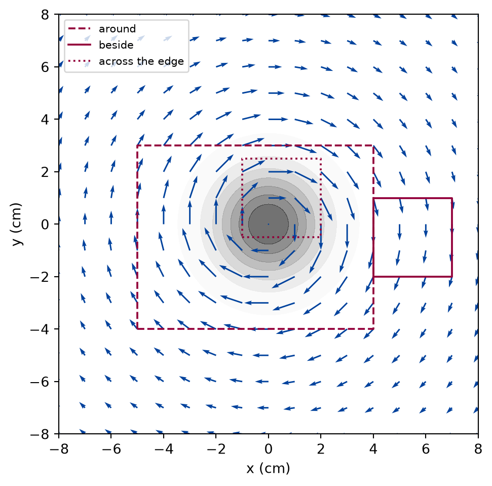
A tube of field of 2 cm width along $z$ grows at 10 T/s. Three square loops lie at rest in the plane across it: one around the tube, one beside it, and one across its edge. Their EMF is the line integral of the induced electric field alone, and is compared with minus the rate of change of their flux.

TUBE = 0.02  # m
RATE = 10.0  # T/s
loops = {
    "around": Rectangle([-0.05, -0.04, 0.0], [0.09, 0.0, 0.0], [0.0, 0.07, 0.0]),
    "beside": Rectangle([0.04, -0.02, 0.0], [0.03, 0.0, 0.0], [0.0, 0.03, 0.0]),
    "across the edge": Rectangle(
        [-0.01, -0.005, 0.0], [0.03, 0.0, 0.0], [0.0, 0.03, 0.0]
    ),
}

src/pbc/electromagnetism/experiments/faradays_law_and_induction.py, lines 197 to 205, read from the repository when this page was built.

def tube_magnetic_at(t):
    return lambda p: flux_tube_fields(
        p, strength=1.0 + RATE * t, rate=RATE, width=TUBE
    )[1]

src/pbc/electromagnetism/experiments/faradays_law_and_induction.py, lines 209 to 212, read from the repository when this page was built.

def tube_electric(p):
    return flux_tube_fields(p, strength=1.0, rate=RATE, width=TUBE)[0]

src/pbc/electromagnetism/experiments/faradays_law_and_induction.py, lines 215 to 216, read from the repository when this page was built.

def tube_run(experiment: Experiment) -> list[tuple[str, float, float, float]]:
    """For each loop at rest, the line integral of the induced field against
    minus the rate of its flux, and the strongest induced field on its wire;
    record the table, return its rows."""
    rows = []
    for name, loop in loops.items():
        induced = emf(loop, electric=tube_electric, nodes=48)
        change = flux_rate(
            lambda t, loop=loop: flux(tube_magnetic_at(t), loop, nodes=48), 0.0, 1e-3
        )
        points, _ = loop.edge(48)
        strongest = float(np.max(np.linalg.norm(tube_electric(points), axis=-1)))
        assert abs(induced + change) <= FARADAY_TOLERANCE * abs(RATE * np.pi * TUBE**2)
        rows.append((name, induced * 1e3, -change * 1e3, strongest * 1e3))

    experiment.table(
        "tube-run",
        rows,
        [
            ("loop", "", ""),
            ("EMF along the wire", "mV", ".5f"),
            ("minus the rate of the flux", "mV", ".5f"),
            ("strongest induced field on the wire", "mV/m", ".2f"),
        ],
        "For three loops at rest near a growing tube of field: the EMF from the "
        "induced electric field along the wire, minus the rate of change of the "
        "flux through the loop, and the strongest induced field on the wire, to "
        "the stated decimals.",
    )
    return rows

src/pbc/electromagnetism/experiments/faradays_law_and_induction.py, lines 219 to 248, read from the repository when this page was built.

For three loops at rest near a growing tube of field: the EMF from the induced electric field along the wire, minus the rate of change of the flux through the loop, and the strongest induced field on the wire, to the stated decimals.
loop	EMF along the wire (mV)	minus the rate of the flux (mV)	strongest induced field on the wire (mV/m)
around	-12.29268	-12.29268	59.63
beside	-0.02003	-0.02003	49.08
across the edge	-5.13583	-5.13583	63.82

def draw_tube() -> Figure:
    """The induced field around the tube, the tube shaded, and the three
    loops."""
    lim = 0.08
    gx, gy = np.meshgrid(np.linspace(-lim, lim, 17), np.linspace(-lim, lim, 17))
    plane = np.stack([gx, gy, np.zeros_like(gx)], axis=-1)
    arrows = tube_electric(plane)
    fx, fy = np.meshgrid(np.linspace(-lim, lim, 201), np.linspace(-lim, lim, 201))
    shade = flux_tube_fields(
        np.stack([fx, fy, np.zeros_like(fx)], axis=-1),
        strength=1.0,
        rate=RATE,
        width=TUBE,
    )[1][..., 2]
    fig, ax = plt.subplots(figsize=(5.6, 5.6))
    ax.contourf(
        fx * 100,
        fy * 100,
        shade,
        levels=np.linspace(0.05, 1.0, 8),
        cmap="Greys",
        alpha=0.6,
    )
    ax.quiver(
        gx * 100, gy * 100, arrows[..., 0], arrows[..., 1], color=FIGURE_COLOURS[0]
    )
    for (name, loop), style in zip(loops.items(), ["--", "-", ":"], strict=True):
        corners = np.array(
            [
                loop.corner,
                loop.corner + loop.side_a,
                loop.corner + loop.side_a + loop.side_b,
                loop.corner + loop.side_b,
                loop.corner,
            ]
        )
        ax.plot(
            corners[:, 0] * 100,
            corners[:, 1] * 100,
            linestyle=style,
            color=FIGURE_COLOURS[1],
            linewidth=1.4,
            label=name,
        )
    ax.set_aspect("equal")
    ax.set_xlabel("x (cm)")
    ax.set_ylabel("y (cm)")
    ax.legend(fontsize=8, loc="upper left")
    return fig

src/pbc/electromagnetism/experiments/faradays_law_and_induction.py, lines 251 to 299, read from the repository when this page was built.

A square plot of the plane across the tube. A grey disc at the centre shades the tube of magnetic field. Arrows circle it clockwise, longest a little outside the disc and shrinking slowly with the distance. A large dashed square surrounds the disc, a small solid square sits to the right of it in the region of arrows only, and a dotted square, off centre, covers part of the disc and its centre. — Figure 2: simulated The induced electric field (arrows) circulates around a growing tube of magnetic field (shaded), and is still strong where the magnetic field has fallen to nothing. The three loops of the table: the large one encloses the tube, the small one beside it encloses almost none of its flux, and the third, off centre, cuts through the tube.

Numerically verified (square loops at rest near a smooth tube of field that grows at a constant rate, induced field from the vector potential): For a loop at rest in a changing magnetic field, the line integral of the induced electric field around the loop equals minus the rate of change of the flux through it, for a loop around the field, beside it, and across its edge. In each row the EMF and minus the rate of the flux agree, to the chosen tolerance of 1e-06 of the rate of the whole flux of the tube, 12.5664 mV. The loop around the tube picks up nearly all of that, though on its wire the magnetic field is practically zero: the EMF counts the flux inside, not the field on the wire. The loop beside the tube sits in an induced field nearly as strong as on the others, as the last column shows, yet its EMF is 0.16 per cent of the first one’s, the share of the flux of the tube that leaks into it. The field pushes the charges forward on one side of that loop and back on the other. The data are simulated, and the check is the flux rule.

Limits

No current. The loops are open, or have no resistance to speak of. A current would add a field of its own, opposing the change, and for a superconducting loop it would keep the flux constant. The lesson computes the EMF, not the current.
Rigid loops. The examples move a loop without changing its shape. A loop that stretches, a sliding bar on rails, follows the same rule, as the first exercise shows; a loop whose material is not a single wire, such as a disc that turns, is where the flux rule needs care.
Given fields, slow changes. The fields are prescribed in closed form. When they change fast enough for light to take a noticeable fraction of a period to cross the loop, the fields become waves, and this description with a single time is no longer exact.
Smooth fields. The field of a real coil drops sharply at its wall, and a quadrature across that wall would converge slowly; the tube of the third example is smooth on purpose.

Self-check. A long coil carries a current that grows, so the field inside it grows. A wire loop goes around the coil, far outside it, where the magnetic field is practically zero. Is there an EMF around the loop?

No. The wire is where the magnetic field is zero, so nothing acts on its charges.

The magnetic field on the wire is nearly zero, but the induced electric field is not: it circulates around the coil and falls only slowly with the distance. That field pushes the charges along the wire.
Yes. The EMF is minus the rate of change of the flux inside the loop, and the loop encloses the growing flux of the coil.

Correct: the loop around the tube in the third example shows it. The force on the charges is the induced electric field, which is there even where the magnetic field is not.
Only if the loop moves, since there is no $\mathbf{u}\times\mathbf{B}$ on a wire at rest.

A loop at rest feels the induced electric field. The motional term is one of two ways for the flux to change, not the only one.

Solution to the self-check

Yes. The flux through the loop is the flux of the coil, and it grows, so the EMF is minus its rate of change, whatever the size or the shape of the loop as long as it goes around the coil once. What pushes the charges is the induced electric field, which circulates around the coil and reaches the wire though the magnetic field there is practically zero.

Exercises

Exercise 1. A bar sliding on rails. Two rails 10 cm apart lie in a uniform field of 0.2 T at right angles to their plane. A bar slides along them at 3 m/s and closes the loop. Compute the EMF from the force on the charges of the moving bar, and compare it with minus the rate of the flux through the growing loop and with $B L v$ .

Hint 1 of 1 for exercise 1

Only the bar moves. The flux is the field times an area that grows by the gap times the speed per unit time.

Solution to exercise 1

def sliding_bar() -> tuple[float, float, float]:
    """Exercise 1: the EMF of a bar sliding on rails, from the force on its
    charges, from minus the rate of the flux, and B L v."""
    b_rails = np.array([0.0, 0.0, 0.2])
    gap, bar_speed, start = 0.1, 3.0, 0.5

    def rails(t):
        return Rectangle(
            [0.0, 0.0, 0.0], [start + bar_speed * t, 0.0, 0.0], [0.0, gap, 0.0]
        )

    def bar_only(points):
        # the bar is the side at the far end; the rest of the loop is at rest
        moving = np.isclose(points[..., 0], start)
        return np.where(moving[..., None], [bar_speed, 0.0, 0.0], 0.0)

    bar_emf = emf(rails(0.0), magnetic=uniform(b_rails), velocity=bar_only)
    rails_rate = -flux_rate(lambda t: flux(uniform(b_rails), rails(t)), 0.0, 1e-4)
    blv = b_rails[2] * gap * bar_speed
    return bar_emf, rails_rate, blv

src/pbc/electromagnetism/experiments/faradays_law_and_induction.py, lines 302 to 321, read from the repository when this page was built.

The force on the charges of the bar gives -60.0000 mV, minus the rate of the flux -60.0000 mV, and $BLv$ is 60.0000 mV in size. The sign is negative because the loop runs counterclockwise about the field and its flux grows: a current would flow clockwise, and the field of that current would oppose the growth.

Exercise 2. A generator of many turns. A coil of 200 turns of 5 cm by 8 cm turns at 25 Hz in a field of 0.1 T. What is the peak voltage between its ends?

Hint 1 of 1 for exercise 2

Each turn has the EMF of the second example, and the turns are in series.

Solution to exercise 2

def many_turns() -> tuple[float, float]:
    """Exercise 2: the peak EMF of one turn of the coil of 5 cm by 8 cm at
    25 Hz in 0.1 T, and of 200 turns in series."""
    one_turn = dict(angular_velocity=2 * np.pi * 25.0, width=0.05, height=0.08)
    quarter = 0.25 / 25.0  # a quarter of a turn, when the EMF is largest
    single = emf(
        rotating_coil(quarter, **one_turn),
        magnetic=uniform([0.1, 0.0, 0.0]),
        velocity=lambda p: np.cross([0.0, 0.0, one_turn["angular_velocity"]], p),
    )
    return single, 200 * single

src/pbc/electromagnetism/experiments/faradays_law_and_induction.py, lines 324 to 334, read from the repository when this page was built.

One turn gives 0.0628 V at its peak, a quarter of a turn after it faces the field, so the coil gives 12.566 V, the formula $N B A \omega$ .

Exercise 3. How wide is beside? Move the loop beside the tube of the third example further out, in steps of 1 cm, and compute its EMF. How does it fall, and why does the induced field on the wire fall more slowly?

Hint 1 of 1 for exercise 3

Compare the flux of the tube that reaches the loop with the strength of the induced field at its distance.

Solution to exercise 3

def further_out(experiment: Experiment) -> tuple[list[float], list[float]]:
    """Exercise 3: the EMF, the rate of the flux, and the strongest induced
    field of the square beside the tube, moved out in steps of 1 cm; record
    the table, return the EMFs and the fields."""
    offsets = np.arange(0.04, 0.09, 0.01)
    beside_emf = []
    beside_rate = []
    beside_field = []
    for x0 in offsets:
        square = Rectangle([x0, -0.02, 0.0], [0.03, 0.0, 0.0], [0.0, 0.03, 0.0])
        beside_emf.append(abs(emf(square, electric=tube_electric, nodes=48)))
        beside_rate.append(
            abs(
                flux_rate(
                    lambda t, square=square: flux(
                        tube_magnetic_at(t), square, nodes=48
                    ),
                    0.0,
                    1e-3,
                )
            )
        )
        points, _ = square.edge(48)
        beside_field.append(
            float(np.max(np.linalg.norm(tube_electric(points), axis=-1)))
        )
    experiment.table(
        "further-out",
        [
            (x0 * 100, e * 1e3, r * 1e3, f * 1e3)
            for x0, e, r, f in zip(
                offsets, beside_emf, beside_rate, beside_field, strict=True
            )
        ],
        [
            ("near side at", "cm", ".0f"),
            ("size of the EMF", "mV", ".2e"),
            ("size of the rate of the flux", "mV", ".2e"),
            ("strongest field on the wire", "mV/m", ".2f"),
        ],
        "The size of the EMF of the small square beside the growing tube, the "
        "size of the rate of change of its flux, and the strongest induced field "
        "on its wire, for each distance of its near side from the axis, to three "
        "significant digits.",
    )
    return beside_emf, beside_field

src/pbc/electromagnetism/experiments/faradays_law_and_induction.py, lines 337 to 382, read from the repository when this page was built.

The size of the EMF of the small square beside the growing tube, the size of the rate of change of its flux, and the strongest induced field on its wire, for each distance of its near side from the axis, to three significant digits.
near side at (cm)	size of the EMF (mV)	size of the rate of the flux (mV)	strongest field on the wire (mV/m)
4	2.00e-02	2.00e-02	49.08
5	1.74e-03	1.74e-03	39.92
6	9.46e-05	9.46e-05	33.33
7	3.18e-06	3.18e-06	28.57
8	6.60e-08	6.60e-08	25.00

The EMF and the rate of the flux agree in every row, and fall by orders of magnitude, from 2.0e-02 mV to 6.6e-08 mV, as fast as the tail of the field of the tube that still reaches the square. The induced field on the wire falls only as the inverse of the distance, from 49.1 to 25.0 mV/m. The field on the wire is strong, but around a loop that encloses almost no flux it pushes the charges forward on one side as much as it holds them back on the other.

Run this experiment

This page was built from commit 6417e2ff90258bd2d2ba21d217eb7666fd24f680 of the repository.

In a clone at that commit, with the project’s Python packages installed, this command runs the experiment of this page:

uv run --locked --no-dev python -m pbc.electromagnetism.experiments.faradays_law_and_induction results

Files, tests, and every command

The files behind it:

site/lessons/electromagnetism/03-faradays-law-and-induction/index.qmd: this page, with every code cell.
src/pbc/electromagnetism/induction.py: code the experiment runs.
src/pbc/electromagnetism/experiments/faradays_law_and_induction.py: code the experiment runs.
src/pbc/experiment.py: code the experiment runs.
tests/unit/test_electromagnetism.py: tests of that code.
tests/unit/test_faradays_law_and_induction_experiment.py: tests of that code.

With Git and uv installed (see the setup page), run:

git clone https://github.com/taspinar/physics-by-construction.git
cd physics-by-construction
git checkout 6417e2ff90258bd2d2ba21d217eb7666fd24f680
uv sync --locked --no-dev
uv run --locked --no-dev python -m pbc.electromagnetism.experiments.faradays_law_and_induction results

The experiment writes every figure of this page into results/, as <label>.png, and every number and table of the page, as the page shows it, into results/results.json. Its numbers match this page to the digits shown, and its figure files are the ones the page shows; digits beyond those can differ between machines, because floating-point libraries differ. Change the code of the experiment and run it again to see what changes.