Charged particles in electric and magnetic fields

The Lorentz force integrated with the Boris pusher: a proton circles in a magnetic field at the cyclotron frequency and the Larmor radius, keeps its energy where explicit Euler does not, and drifts across crossed fields at E over B, each checked against its formula.

Course

Electromagnetism, lesson 2 of 3

Slot

EM2, Lorentz force and charged particles

Methods

Simulation

Difficulty

Intermediate, level 2 of 3

What you’ll learn

Integrate the motion of a charged particle under the Lorentz force with the Boris pusher
Measure the cyclotron frequency and the Larmor radius of a simulated orbit and check them against qB/m and mv/(qB)
Predict the error of the Boris pusher from its own closed form and measure its order
Explain why explicit Euler gains energy in a magnetic field, and compute the drift of a particle in crossed fields

Prerequisites

Electric fields, superposition, and the potential, Numerical integrators.

Before you begin

Vectors: the cross product in three dimensions
Trigonometry: the tangent of a half angle

Related

none

Previous

Electric fields, superposition, and the potential

Next

Induction: magnetic flux and the electromotive force

With scripts, this page keeps a record in your browser of whether you completed the lesson. Nothing is stored without them.

With scripts, this place suggests what to do next, with the reason, from the progress saved in your browser. Without them, follow the learning path.

A beam of protons in an accelerator is steered around a ring by magnets. The aurora shines where electrons from the Sun spiral down the field lines of the Earth into the air. A mass spectrometer sorts ions by the size of the circle a magnetic field bends them into. All three rest on one force: a charge that moves through a magnetic field is pushed sideways, at right angles to its velocity and to the field, and an electric field pushes it along.

The previous lesson computed the electric field of charges at rest. This one takes the fields as given and asks how a charge moves in them. How fast does a proton circle in a uniform magnetic field, and how large is its circle? What does an electric field across the magnetic one add? And how is such a motion computed, so that a simulation of millions of turns does not slowly invent energy that the force cannot give? The motion is integrated with the Boris pusher, the method of most plasma codes, and the frequency, the radius, and the drift are measured from the simulated orbit and compared with their formulas. The formulas are not used to compute the orbit.

Assumptions

Given fields. The electric and magnetic fields are set from outside and do not change with the particle. The particle’s own field, and its effect on the charges that make the fields, are ignored. In a plasma, with many particles, the fields come from the particles too, and this is no longer true.
Slow compared with light. The momentum is $m\mathbf{v}$ , with a constant mass. At a speed $v$ the relativistic correction is of order $(v/c)^2$ ; for the speeds of the lesson it is below a part in ten million. An electron in a television tube or a proton in an accelerator needs the relativistic form.
No radiation. A charge on a circle accelerates, and an accelerated charge radiates and loses energy. For a proton in a field of a tesla the loss is far too slow to matter over the times computed; for electrons in a storage ring it is the main effect.
Uniform fields. The examples use fields that are the same everywhere. A field that changes over the size of the orbit makes the centre of the circle drift as well; that is the physics of magnetic mirrors and of the radiation belts, and is not in this lesson.
A fixed time step. The pusher takes steps of one size. Its error is set by the angle the velocity turns in one step, so the step is chosen as a fraction of the period of the circle.

The Lorentz force and the Boris pusher

The force

A charge $q$ of mass $m$ in an electric field $\mathbf{E}$ and a magnetic field $\mathbf{B}$ feels the Lorentz force,

$m\,\frac{\mathrm{d}\mathbf{v}}{\mathrm{d}t} = q\left(\mathbf{E} + \mathbf{v}\times\mathbf{B}\right).$

The magnetic part is at right angles to the velocity, so it does no work: $\mathbf{v}\cdot(\mathbf{v}\times\mathbf{B}) = 0$ , and the speed stays the same. In a uniform field $\mathbf{B} = B\,\hat{\mathbf{z}}$ with no electric field, the velocity across the field turns at a constant rate, and the particle runs on a circle. The rate is the cyclotron frequency, and the radius the Larmor radius,

$\omega_c = \frac{|q|\,B}{m}, \qquad r_L = \frac{m\,v_\perp}{|q|\,B} = \frac{v_\perp}{\omega_c},$

with $v_\perp$ the speed across the field. The frequency does not depend on the speed: a fast particle runs on a larger circle in the same time, which is why a cyclotron can accelerate with a voltage of a fixed frequency. The motion along the field is not affected, so in general the orbit is a helix. A positive charge turns clockwise seen from the tip of $\mathbf{B}$ , a negative one counterclockwise.

Crossed fields

Add a uniform electric field at right angles to $\mathbf{B}$ . In a frame that moves with the velocity

$\mathbf{v}_d = \frac{\mathbf{E}\times\mathbf{B}}{B^2}$

the electric field vanishes (to the order of the assumptions), and the particle circles again. In the frame of the lab the centre of the circle drifts with $\mathbf{v}_d$ : at right angles to both fields, at the speed $E/B$ , and in the same direction for a positive and a negative charge, since both $q$ and the sense of the turn change sign together.

The Boris pusher

The pusher keeps the position at whole steps and the velocity half a step later, as the leapfrog method of the mechanics course does. A step of length $\Delta t$ is

half a kick by the electric field: $\mathbf{v}^- = \mathbf{v}_{n-1/2} + \tfrac{q}{m}\mathbf{E}\,\tfrac{\Delta t}{2}$ ;
a rotation of $\mathbf{v}^-$ about $\mathbf{B}$ to $\mathbf{v}^+$ , with $\mathbf{t} = \tfrac{q}{m}\mathbf{B}\,\tfrac{\Delta t}{2}$ and $\mathbf{s} = 2\mathbf{t}/(1 + t^2)$ : $\mathbf{v}' = \mathbf{v}^- + \mathbf{v}^-\times\mathbf{t}$ and $\mathbf{v}^+ = \mathbf{v}^- + \mathbf{v}'\times\mathbf{s}$ ;
the second half kick, $\mathbf{v}_{n+1/2} = \mathbf{v}^+ + \tfrac{q}{m}\mathbf{E}\,\tfrac{\Delta t}{2}$ ;
the drift, $\mathbf{x}_{n+1} = \mathbf{x}_n + \Delta t\,\mathbf{v}_{n+1/2}$ .

The second step is an exact rotation: it keeps the length of the velocity to round-off, so in a magnetic field the pusher keeps the energy for any number of steps, as the force does. The angle of the rotation is not $\omega_c\Delta t$ but $\theta$ with

$\tan\frac{\theta}{2} = \frac{\omega_c\,\Delta t}{2},$

so that the pusher circles at its own frequency $\omega_B = \theta/\Delta t$ , a little slower than $\omega_c$ by $\omega_c^3\Delta t^2/12$ to the lowest order. Its positions are the corners of a regular polygon with the side $v_\perp\Delta t$ and the angle $\theta$ between sides, which lie on a circle of radius

$r_B = \frac{v_\perp\,\Delta t}{2\sin(\theta/2)} = r_L\,\sqrt{1 + \left(\frac{\omega_c\Delta t}{2}\right)^2}.$

Both converge to the true values as $\Delta t^2$ : the Boris pusher is of second order, and its error is known in closed form, which lets the lesson check the simulation twice, against the physics and against the method.

Explicit Euler

Explicit Euler advances the velocity with the force at the start of the step, $\mathbf{v}_{n+1} = \mathbf{v}_n + \tfrac{q}{m}\Delta t\,\mathbf{v}_n\times\mathbf{B}$ . The change is at right angles to $\mathbf{v}_n$ , so by Pythagoras $|\mathbf{v}_{n+1}|^2 = |\mathbf{v}_n|^2\,(1 + (\omega_c\Delta t)^2)$ for a velocity across the field: every step multiplies the kinetic energy by the same factor larger than one, and the particle spirals outwards.

Code

The pusher is boris; the lines of the rotation are the heart of it. The frequency is read from the simulated velocity by measured_angular_frequency, the slope of its angle in time, and the radius by fitted_radius, a least-squares circle through the positions.

        turn = half * magnetic(x[n], t[n])
        scale = 2.0 / (1.0 + turn @ turn)
        minus = v[n] + kick
        prime = minus + np.cross(minus, turn)
        plus = minus + scale * np.cross(prime, turn)

Line 94, turn = half * magnetic(x[n], t[n]): The vector t of the explanation: the field times half the step and the charge over the mass.
Line 97, prime = minus + np.cross(minus, turn): The first half of the rotation; with the next line it turns the velocity without changing its length.

src/pbc/electromagnetism/motion.py, lines 94 to 98, read from the repository when this page was built.

def boris_frequency(omega: float, dt: float) -> float:
    """The angular frequency of the gyration that the Boris pusher computes
    at the true frequency ``omega`` (rad/s) and the step ``dt`` (s):
    2 arctan(omega dt / 2) / dt, below omega by omega^3 dt^2 / 12 to the
    lowest order."""
    return 2.0 * np.arctan(0.5 * omega * dt) / dt

src/pbc/electromagnetism/motion.py, lines 144 to 149, read from the repository when this page was built.

def measured_angular_frequency(
    t: ArrayLike, v: ArrayLike, *, drift: ArrayLike = (0.0, 0.0, 0.0)
) -> float:
    """The rate (rad/s) at which the velocity, less ``drift``, turns in the
    x-y plane: the slope of its unwrapped angle against the time, fitted by
    least squares. Positive whatever the sense of the turn."""
    t = np.asarray(t, dtype=float)
    u = np.asarray(v, dtype=float) - np.asarray(drift, dtype=float)
    angle = np.unwrap(np.arctan2(u[:, 1], u[:, 0]))
    return float(abs(np.polyfit(t, angle, 1)[0]))

src/pbc/electromagnetism/motion.py, lines 175 to 184, read from the repository when this page was built.

Worked examples

A proton in a uniform magnetic field

A proton moves at 100 km/s across a uniform field of 1 T. It is followed for ten turns with steps of a twentieth of the period down to a three-hundred-and-twentieth, and the frequency and the radius of the simulated orbit are measured.

FIELD = np.array([0.0, 0.0, 1.0])  # T
SPEED = 1e5  # m/s
OMEGA = cyclotron_frequency(PROTON_CHARGE_TO_MASS, FIELD[2])  # rad/s
RADIUS = larmor_radius(PROTON_CHARGE_TO_MASS, FIELD[2], SPEED)  # m
PERIOD = 2 * np.pi / OMEGA  # s
METHOD_TOLERANCE = 1e-10  # a chosen tolerance against the pusher's own closed form
per_period = np.array([20, 40, 80, 160, 320])

src/pbc/electromagnetism/experiments/charged_particles_in_fields.py, lines 42 to 48, read from the repository when this page was built.

def cyclotron_run(experiment: Experiment) -> tuple[list[float], float]:
    """The frequency and radius of ten simulated turns for each step, against
    the pusher's closed forms and against qB/m and mv/(qB); record the table,
    return the gaps of the frequency and their fitted order."""
    rows = []
    gaps = []
    for n in per_period:
        dt = PERIOD / n
        orbit = boris(
            NO_FIELD,
            [SPEED, 0.0, 0.0],
            q_over_m=PROTON_CHARGE_TO_MASS,
            electric=NO_FIELD,
            magnetic=FIELD,
            dt=dt,
            n_steps=10 * n,
        )
        omega = measured_angular_frequency(orbit.t, orbit.v)
        radius = fitted_radius(orbit.x)
        assert abs(omega / boris_frequency(OMEGA, dt) - 1) < METHOD_TOLERANCE
        assert abs(radius / boris_radius(OMEGA, dt, SPEED) - 1) < METHOD_TOLERANCE
        gaps.append(abs(omega / OMEGA - 1))
        rows.append(
            (n, omega / OMEGA, boris_frequency(OMEGA, dt) / OMEGA, radius / RADIUS)
        )
    order = fitted_order(PERIOD / per_period, gaps)
    assert abs(order - 2.0) < 0.02, "the pusher is not of second order"

    experiment.table(
        "cyclotron-run",
        rows,
        [
            ("steps per period", "", "d"),
            ("measured frequency over qB/m", "", ".8f"),
            ("Boris frequency over qB/m", "", ".8f"),
            ("measured radius over mv/(qB)", "", ".8f"),
        ],
        "The angular frequency and the radius of the simulated orbit of a "
        "proton, measured from ten turns, as fractions of the cyclotron "
        "frequency and the Larmor radius, with the frequency the Boris pusher "
        "predicts for its step, to eight decimals.",
    )
    return gaps, order

src/pbc/electromagnetism/experiments/charged_particles_in_fields.py, lines 67 to 109, read from the repository when this page was built.

The angular frequency and the radius of the simulated orbit of a proton, measured from ten turns, as fractions of the cyclotron frequency and the Larmor radius, with the frequency the Boris pusher predicts for its step, to eight decimals.
steps per period	measured frequency over qB/m	Boris frequency over qB/m	measured radius over mv/(qB)
20	0.99189499	0.99189499	1.01226183
40	0.99795141	0.99795141	1.00307951
80	0.99948643	0.99948643	1.00077077
160	0.99987152	0.99987152	1.00019275
320	0.99996787	0.99996787	1.00004819

Numerically verified (a non-relativistic proton, a uniform field, ten turns, steps from a twentieth of a period down): A proton in a uniform magnetic field circles at the cyclotron frequency $qB/m$ on the Larmor radius $mv/(qB)$ ; the frequency and the radius of the Boris orbit converge to both with order two in the step, and agree with the pusher’s own closed forms to round-off. The cyclotron frequency of the proton is 9.5788e+07 rad/s, a turn every 65.59 ns, and the Larmor radius is 1.044 mm. With a twentieth of the period per step the pusher runs 0.81 per cent slow, and with the finest step the gap is 3.2e-05; the fitted order of the gap is 1.995. The measured frequency and radius match the closed forms of the pusher, $\omega_B$ and $r_B$ , to within 1e-10 at every step: the error of the simulation is not noise, it is the known error of the method.

Why the energy matters: Boris against explicit Euler

The same proton is followed for five turns with eighty steps per turn, once with the Boris pusher and once with explicit Euler.

steps_per_turn = 80
turns = 5
ENERGY_FLOOR = 1e-12  # a bound shown in place of a value at round-off

src/pbc/electromagnetism/experiments/charged_particles_in_fields.py, lines 52 to 54, read from the repository when this page was built.

def energy_run(experiment: Experiment) -> tuple[Trajectory, Trajectory, float]:
    """Five turns of eighty steps with Boris and with explicit Euler, and the
    energy of each against the start; record the table, return both orbits
    and the final energy of Euler over the initial."""
    dt = PERIOD / steps_per_turn
    pushed = boris(
        NO_FIELD,
        [SPEED, 0.0, 0.0],
        q_over_m=PROTON_CHARGE_TO_MASS,
        electric=NO_FIELD,
        magnetic=FIELD,
        dt=dt,
        n_steps=turns * steps_per_turn,
    )
    euler = explicit_euler(
        NO_FIELD,
        [SPEED, 0.0, 0.0],
        q_over_m=PROTON_CHARGE_TO_MASS,
        electric=NO_FIELD,
        magnetic=FIELD,
        dt=dt,
        n_steps=turns * steps_per_turn,
    )
    boris_energy = np.sum(pushed.v**2, axis=1) / SPEED**2
    euler_energy = np.sum(euler.v**2, axis=1) / SPEED**2
    predicted = euler_energy_factor(OMEGA, dt) ** np.arange(len(euler_energy))
    boris_drift = float(np.max(np.abs(boris_energy - 1.0)))
    assert boris_drift < ENERGY_FLOOR, "the Boris pusher changed the energy"
    assert np.allclose(euler_energy, predicted, rtol=1e-10), (
        "Euler did not grow as predicted"
    )

    experiment.table(
        "energy-run",
        [
            ("Boris", f"below {ENERGY_FLOOR:.0e}", None),
            ("explicit Euler", f"{euler_energy[-1]:.4f}", predicted[-1]),
        ],
        [
            ("method", "", ""),
            ("final energy over initial", "", ""),
            ("predicted by the factor per step", "", ".4f"),
        ],
        "The kinetic energy after five turns of eighty steps, relative to the "
        "start, for each method (for Boris the change from one), and the "
        "growth that the factor of explicit Euler per step predicts.",
    )
    return pushed, euler, float(euler_energy[-1])

src/pbc/electromagnetism/experiments/charged_particles_in_fields.py, lines 112 to 159, read from the repository when this page was built.

The kinetic energy after five turns of eighty steps, relative to the start, for each method (for Boris the change from one), and the growth that the factor of explicit Euler per step predicts.
method	final energy over initial	predicted by the factor per step
Boris	below 1e-12
explicit Euler	11.7027	11.7027

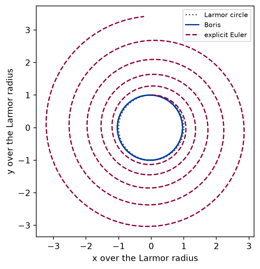
def draw_gyration(pushed: Trajectory, euler: Trajectory) -> Figure:
    """The Boris and the Euler orbits against the Larmor circle, in units of
    the Larmor radius."""
    centre = np.array([0.0, -RADIUS])  # a proton moving along x turns towards -y
    angle = np.linspace(0, 2 * np.pi, 361)
    fig, ax = plt.subplots(figsize=(5.6, 5.0))
    ax.plot(
        np.cos(angle),
        np.sin(angle),
        color=FIGURE_COLOURS[2],
        linestyle=":",
        label="Larmor circle",
    )
    ax.plot(
        (pushed.x[:, 0] - centre[0]) / RADIUS,
        (pushed.x[:, 1] - centre[1]) / RADIUS,
        color=FIGURE_COLOURS[0],
        label="Boris",
    )
    ax.plot(
        (euler.x[:, 0] - centre[0]) / RADIUS,
        (euler.x[:, 1] - centre[1]) / RADIUS,
        color=FIGURE_COLOURS[1],
        linestyle="--",
        label="explicit Euler",
    )
    ax.set_aspect("equal")
    ax.set_xlabel("x over the Larmor radius")
    ax.set_ylabel("y over the Larmor radius")
    ax.legend(fontsize=8, loc="upper right")
    return fig

src/pbc/electromagnetism/experiments/charged_particles_in_fields.py, lines 162 to 192, read from the repository when this page was built.

Plot of the orbit in the plane across the field, in units of the Larmor radius. A dotted circle marks the exact orbit. The solid blue Boris orbit lies on it, turn after turn. The dashed red Euler orbit starts on the circle and spirals outwards in widening loops. — Figure 1: simulated Five turns of a proton in a uniform magnetic field with eighty steps per turn. The Boris orbit (blue, solid) stays on the circle of the Larmor radius (dotted); explicit Euler (red, dashed) spirals outwards, gaining energy at every step.

Numerically verified (a uniform magnetic field, eighty steps per turn, five turns): In a magnetic field the Boris pusher keeps the kinetic energy to round-off, while explicit Euler multiplies it by $1 + (\omega_c\Delta t)^2$ at every step. After five turns explicit Euler has multiplied the energy by 11.70, the factor that the growth per step predicts, and its orbit has left the circle, as the figure shows. The Boris energy has moved by less than 1e-12. The two methods take the same steps and the same force; what differs is that the rotation of Boris is a rotation, and the step of Euler is not.

Crossed fields: the drift

A field of 10 kV/m along $y$ is added to the field of 1 T along $z$ . A proton and an electron start at rest and are followed for fifty turns of fifty steps each. The electron is put in fields a thousand times weaker, both of them, so that $E/B$ is the same and its circle is not too small to draw. The velocity of the centre of each orbit is fitted and compared with $\mathbf{E}\times\mathbf{B}/B^2$ .

ELECTRIC = np.array([0.0, 1e4, 0.0])  # V/m
DRIFT_TOLERANCE = 1e-8  # a chosen tolerance, relative to the drift speed
particles = [
    ("proton", PROTON_CHARGE_TO_MASS, 1.0),
    ("electron", ELECTRON_CHARGE_TO_MASS, 1e-3),
]

src/pbc/electromagnetism/experiments/charged_particles_in_fields.py, lines 58 to 63, read from the repository when this page was built.

def drift_run(experiment: Experiment) -> dict[str, tuple[Trajectory, float]]:
    """A proton and an electron from rest in crossed fields for fifty turns,
    the fitted velocity of the centre against E x B / B^2; record the table,
    return each orbit and its period."""
    rows = []
    orbits = {}
    for name, q_over_m, b in particles:
        magnetic = np.array([0.0, 0.0, b])
        electric = ELECTRIC * b  # keeps E/B, and so the drift, the same
        expected = drift_velocity(electric, magnetic)
        period = 2 * np.pi / cyclotron_frequency(q_over_m, b)
        dt = period / 50
        orbit = boris(
            NO_FIELD,
            NO_FIELD,
            q_over_m=q_over_m,
            electric=electric,
            magnetic=magnetic,
            dt=dt,
            n_steps=50 * 50,
        )
        omega = measured_angular_frequency(orbit.t, orbit.v, drift=expected)
        found = guiding_centre_velocity(orbit.t, orbit.x, omega)
        gap = float(np.linalg.norm(found - expected) / np.linalg.norm(expected))
        assert gap < DRIFT_TOLERANCE, f"the {name} does not drift with E x B / B^2"
        orbits[name] = (orbit, period)
        rows.append(
            (
                name,
                b,
                electric[1],
                found[0],
                expected[0],
                f"below {DRIFT_TOLERANCE:.0e}",
            )
        )

    experiment.table(
        "drift-run",
        rows,
        [
            ("particle", "", ""),
            ("magnetic field", "T", ".3f"),
            ("electric field", "V/m", ".0f"),
            ("drift along x", "m/s", ".3f"),
            ("E over B", "m/s", ".3f"),
            ("relative difference of the drift vectors", "", ""),
        ],
        "The velocity of the centre of the orbit of a proton and of an electron "
        "in crossed fields, fitted from fifty turns, against the drift E x B "
        "over B squared, to three decimals, and the relative difference of the "
        "two vectors, given as a bound.",
    )
    return orbits

src/pbc/electromagnetism/experiments/charged_particles_in_fields.py, lines 195 to 248, read from the repository when this page was built.

The velocity of the centre of the orbit of a proton and of an electron in crossed fields, fitted from fifty turns, against the drift E x B over B squared, to three decimals, and the relative difference of the two vectors, given as a bound.
particle	magnetic field (T)	electric field (V/m)	drift along x (m/s)	E over B (m/s)	relative difference of the drift vectors
proton	1.000	10000	10000.000	10000.000	below 1e-08
electron	0.001	10	10000.000	10000.000	below 1e-08

def draw_drift(orbits: dict[str, tuple[Trajectory, float]]) -> Figure:
    """The paths of the proton and the electron over four turns of the
    proton."""
    shown_time = 4 * orbits["proton"][1]  # four turns of the proton
    fig, ax = plt.subplots(figsize=(6.4, 3.2))
    for (name, (orbit, _)), colour, style in zip(
        orbits.items(), FIGURE_COLOURS[:2], ["-", "--"], strict=True
    ):
        shown = orbit.t <= shown_time
        ax.plot(
            orbit.x[shown, 0] * 1e6,
            orbit.x[shown, 1] * 1e6,
            color=colour,
            linestyle=style,
            label=name,
        )
    ax.axhline(0.0, color=FIGURE_COLOURS[2], linewidth=0.6)
    ax.set_aspect("equal")
    ax.set_xlabel("x (μm)")
    ax.set_ylabel("y (μm)")
    ax.legend(fontsize=8, loc="upper left", bbox_to_anchor=(1.0, 1.0))
    return fig

src/pbc/electromagnetism/experiments/charged_particles_in_fields.py, lines 251 to 272, read from the repository when this page was built.

Plot of position across the drift against position along it, in micrometres. The blue proton path is a row of tall arches above the starting line; the red electron path is a row of smaller, more numerous arches below it. Both paths end at the same distance to the right. — Figure 2: simulated A proton (blue, solid) and an electron (red, dashed) that start at rest in crossed fields, over the same time. Both drift along x by the same distance, at right angles to both fields, while turning in opposite senses on opposite sides of the line where they started, which their arcs touch, as a point on a rolling wheel does.

Numerically verified (uniform crossed fields, a drift far slower than light, fifty turns): In crossed uniform fields the centre of the orbit drifts with $\mathbf{E}\times\mathbf{B}/B^2$ , at right angles to both fields and in the same direction for a positive and a negative charge. The fitted drift of both particles agrees with $E/B$ to a relative difference below 1e-08, and points along $x$ for both, though the proton turns clockwise and the electron counterclockwise, as the figure shows. The electron turns faster and on smaller arcs, yet in the same time it covers the same distance along $x$ : the drift depends on the fields alone, not on the charge or the mass. The data are simulated, and the check is the drift formula.

Limits

Non-relativistic. The lesson integrates $m\,\mathrm{d}\mathbf{v}/\mathrm{d}t$ with a constant mass. At a speed close to light the cyclotron frequency falls by the Lorentz factor and the pusher has to advance the momentum instead; the relativistic Boris pusher does that.
Given, uniform fields. A non-uniform field adds drifts of the gradient and of the curvature of the field, and a field that changes in time can heat or trap the particle. None is computed here.
One particle, no radiation. Nothing here makes a field: there is no interaction between particles and no loss to radiation.
The measured frequency is a fit. It is the slope of the angle of the velocity over the whole run, and the radius is a least-squares circle. For an orbit that is not a circle, as Euler’s is not, neither is a property of the orbit, which is why the first table uses the Boris runs alone.

Self-check. A proton circles in a uniform magnetic field. The field is doubled. What happens to its speed, its radius, and the time of a turn?

The speed doubles, because the force is twice as large.

The magnetic force is at right angles to the velocity and does no work, so the speed cannot change, whatever the field.
The speed stays, the radius halves, and a turn takes half the time.

Correct: $r_L = mv/(qB)$ halves and $\omega_c = qB/m$ doubles, while the force does no work and the speed stays.
The speed and the radius stay, and only the time of a turn halves.

With the same speed and twice the frequency, the circle must be half as large: the radius is the speed divided by the frequency.

Solution to the self-check

The speed stays, because the magnetic force is at right angles to the velocity and does no work. The cyclotron frequency $qB/m$ doubles, so a turn takes half as long, and the radius $v/\omega_c$ halves.

Exercises

Exercise 1. A mass spectrometer. Singly charged ions of carbon-12 and carbon-13 (masses 12.000 u and 13.003 u, with 1 u = 1.66054e-27 kg) leave a source at 50 km/s and are bent by a field of 0.5 T. How far apart do they land after half a circle?

Hint 1 of 1 for exercise 1

After half a circle an ion has moved by the diameter of its circle.

Solution to exercise 1

def mass_spectrometer() -> tuple[float, float]:
    """Exercise 1: the diameters of the half circles of singly charged
    carbon-12 and carbon-13 ions at 50 km/s in 0.5 T."""
    unit = 1.66054e-27  # kg
    charge = 1.602176634e-19  # C
    light, heavy = (
        2 * larmor_radius(charge / (mass * unit), 0.5, 5e4) for mass in (12.000, 13.003)
    )
    return light, heavy

src/pbc/electromagnetism/experiments/charged_particles_in_fields.py, lines 275 to 283, read from the repository when this page was built.

The lighter ion lands 2.487 cm from the source and the heavier 2.695 cm, 2.08 mm apart. At the same speed the radius is proportional to the mass, so the difference of the diameters is the difference of the masses in the same proportion: a spectrometer turns a mass into a distance.

Exercise 2. An electron in the field of the Earth. The field of the Earth is about 50 μT. What is the cyclotron frequency of an electron in it, in hertz, and the radius of the circle at 1000 km/s?

Hint 1 of 1 for exercise 2

The frequency in hertz is the angular frequency divided by a full turn.

Solution to exercise 2

def electron_in_the_earths_field() -> tuple[float, float]:
    """Exercise 2: the cyclotron frequency in hertz of an electron in 50 μT,
    and its radius at 1000 km/s."""
    electron_omega = cyclotron_frequency(ELECTRON_CHARGE_TO_MASS, 50e-6)
    electron_radius = larmor_radius(ELECTRON_CHARGE_TO_MASS, 50e-6, 1e6)
    return electron_omega / (2 * np.pi), electron_radius

src/pbc/electromagnetism/experiments/charged_particles_in_fields.py, lines 286 to 291, read from the repository when this page was built.

The electron turns 1.400 million times a second, on a circle of 11.4 cm: the gyration of the electrons of the upper atmosphere is at a frequency of the radio band, and on a circle of the size of a hand.

Exercise 3. A helix. The proton of the first example gets a speed of 30 km/s along the field as well. Simulate about ten turns and measure how far it advances along the field per turn. Compare with the speed along the field times the period.

Hint 1 of 1 for exercise 3

The force has no component along the field, so the speed along it does not change.

Solution to exercise 3

def helix() -> tuple[float, float]:
    """Exercise 3: the advance per turn along the field of the proton with
    30 km/s along it, simulated, and the speed along it times the period."""
    orbit = boris(
        NO_FIELD,
        [SPEED, 0.0, 3e4],
        q_over_m=PROTON_CHARGE_TO_MASS,
        electric=NO_FIELD,
        magnetic=FIELD,
        dt=PERIOD / 80,
        n_steps=800,
    )
    omega = measured_angular_frequency(orbit.t, orbit.v)
    turns_made = omega * orbit.t[-1] / (2 * np.pi)  # the turns of the pusher
    pitch = (orbit.x[-1, 2] - orbit.x[0, 2]) / turns_made
    expected_pitch = 3e4 * 2 * np.pi / omega
    return pitch, expected_pitch

src/pbc/electromagnetism/experiments/charged_particles_in_fields.py, lines 294 to 310, read from the repository when this page was built.

The proton advances 1.9688 mm along the field per turn, and the speed along the field times the period of the simulated turn gives 1.9688 mm. The motion along the field and the circle across it are independent, and together they make a helix: the path of the electrons that spiral down the field lines into an aurora.

Run this experiment

This page was built from commit 6417e2ff90258bd2d2ba21d217eb7666fd24f680 of the repository.

In a clone at that commit, with the project’s Python packages installed, this command runs the experiment of this page:

uv run --locked --no-dev python -m pbc.electromagnetism.experiments.charged_particles_in_fields results

Files, tests, and every command

The files behind it:

site/lessons/electromagnetism/02-charged-particles-in-fields/index.qmd: this page, with every code cell.
src/pbc/electromagnetism/motion.py: code the experiment runs.
src/pbc/electromagnetism/experiments/charged_particles_in_fields.py: code the experiment runs.
src/pbc/verification/estimates.py: code the experiment runs.
src/pbc/experiment.py: code the experiment runs.
tests/unit/test_electromagnetism.py: tests of that code.
tests/unit/test_charged_particles_in_fields_experiment.py: tests of that code.

With Git and uv installed (see the setup page), run:

git clone https://github.com/taspinar/physics-by-construction.git
cd physics-by-construction
git checkout 6417e2ff90258bd2d2ba21d217eb7666fd24f680
uv sync --locked --no-dev
uv run --locked --no-dev python -m pbc.electromagnetism.experiments.charged_particles_in_fields results

The experiment writes every figure of this page into results/, as <label>.png, and every number and table of the page, as the page shows it, into results/results.json. Its numbers match this page to the digits shown, and its figure files are the ones the page shows; digits beyond those can differ between machines, because floating-point libraries differ. Change the code of the experiment and run it again to see what changes.