Electric fields, superposition, and the potential

The electric field of point charges computed by adding Coulomb’s law charge by charge, checked against minus the gradient of the potential, against the closed form of a dipole far away, and against Gauss’s law on a sphere.

Course

Electromagnetism, lesson 1 of 3

Slot

EM1, Coulomb’s law and electric fields

Methods

Simulation

Difficulty

Introductory, level 1 of 3

What you’ll learn

Compute the electric field of a set of point charges as a vector field, by superposition of Coulomb’s law
Obtain the field from the potential by a numerical gradient and measure the order of its error
Check the field of a pair of charges against the closed form of a dipole, and say how fast the two agree with distance
Check Gauss’s law by computing the flux through a sphere around and beside the charges

Prerequisites

Newton’s laws as a first-order system.

Before you begin

Vectors: components, the dot product, and the gradient of a function of the position
Calculus: partial derivatives, and integrals over a surface

Related

none

Previous

Sound, resonance, and the Doppler effect

Next

Charged particles in electric and magnetic fields

With scripts, this page keeps a record in your browser of whether you completed the lesson. Nothing is stored without them.

With scripts, this place suggests what to do next, with the reason, from the progress saved in your browser. Without them, follow the learning path.

Rub a balloon on a jumper and it holds to the wall. Between the balloon and the wall there is nothing to see, yet a force acts across the gap, and it acts on every bit of charge at every place. Physics describes that by a field: an arrow at every point of space that says which force a small test charge would feel there, per unit of its charge. The field is the first example in the course of a vector field, and nearly everything else in electromagnetism is a statement about such fields.

This lesson builds the electric field of charges at rest from a single law, Coulomb’s law for one charge, and one rule, that the fields of several charges add. It then asks three questions of the result. Is the field the slope of a single number, the potential, as the theory says? What does a pair of opposite charges look like from far away, where the theory replaces it by a dipole? And does the field obey Gauss’s law, which says that the flux out through any closed surface counts the charge inside? Each answer is computed by the program and compared with the closed form; none of the closed forms is used to compute the field.

Assumptions

Point charges at rest. Every charge sits at a point and does not move. A moving charge also makes a magnetic field, and a charge that accelerates radiates; neither is in this lesson.
Vacuum. The charges sit in empty space, with the permittivity $\varepsilon_0$ . In a material the field polarises the atoms and the field inside is smaller; a dielectric constant would describe that.
Superposition. The field of several charges is the sum of the fields of each. That is a law of electromagnetism in vacuum, true to every precision measured, and it fails only for fields so strong that the vacuum itself responds, far beyond anything here.
No field at a charge. The field of a point charge grows without bound as the distance falls, and is not defined at the charge itself. The program refuses a point that lies on a charge, and a real charge has a size.
Floating-point numbers. The numerical gradient divides a small difference by a small step. Too small a step loses digits to the round-off, which sets a floor below which the error no longer falls.

Fields from charges

Coulomb’s law and superposition

A charge $q_i$ at the position $\mathbf{r}_i$ makes at the point $\mathbf{r}$ the field

$\mathbf{E}_i(\mathbf{r}) = k\,q_i\,\frac{\mathbf{r} - \mathbf{r}_i}{|\mathbf{r} - \mathbf{r}_i|^3}, \qquad k = \frac{1}{4\pi\varepsilon_0},$

which points away from a positive charge, towards a negative one, and falls with the square of the distance. A test charge $q$ at $\mathbf{r}$ feels the force $q\,\mathbf{E}$ . For several charges the fields add as vectors,

$\mathbf{E}(\mathbf{r}) = \sum_i \mathbf{E}_i(\mathbf{r}).$

That sum is the whole computation of this lesson. The program evaluates it at an array of points at once, so the same function gives a single arrow or the field over a grid.

The potential

Coulomb’s field has a special property: the work it does on a test charge moved between two points does not depend on the path. Then there is a single number at every point, the potential $V$ , whose slope is the field,

$V(\mathbf{r}) = \sum_i \frac{k\,q_i}{|\mathbf{r} - \mathbf{r}_i|}, \qquad \mathbf{E} = -\nabla V .$

A number is easier than an arrow: the potentials of several charges add as numbers, and the field follows by differentiation. The program checks the relation by differentiating $V$ numerically. A central difference of step $h$ along the axis $x$ ,

$\frac{\partial V}{\partial x} \approx \frac{V(x + h) - V(x - h)}{2h},$

has an error that falls as $h^2$ : in the Taylor expansion of $V$ about $x$ the terms of even order cancel in the difference, and the first term left after the derivative is the third derivative times $h^2/6$ .

The dipole

Two charges $+q$ and $-q$ a distance $d$ apart have no net charge, so from far away the field of one nearly cancels that of the other. What is left is the dipole field, set by the moment $\mathbf{p} = q\,\mathbf{d}$ , the vector from the negative to the positive charge times $q$ . With $\hat{\mathbf{n}}$ the unit vector from the middle of the pair towards the point and $r$ the distance,

$\mathbf{E}_{\text{dipole}} = \frac{k}{r^3}\left(3\,(\mathbf{p}\cdot\hat{\mathbf{n}})\,\hat{\mathbf{n}} - \mathbf{p}\right), \qquad V_{\text{dipole}} = \frac{k\,\mathbf{p}\cdot\hat{\mathbf{n}}}{r^2}.$

It falls with the cube of the distance, one power faster than the field of a single charge. The dipole is the first term of an expansion of the field of the pair in powers of $d/r$ . The pair is symmetric about its middle, so the term after the dipole vanishes, and the next one is smaller by $(d/r)^2$ : the field of the pair and the field of the dipole should differ, relative to the field, by an amount that falls as the square of $d/r$ . That is the prediction the lesson tests.

Gauss’s law

The flux of the field out through a closed surface $S$ is the integral of its outward component over the surface. Gauss’s law says that it counts the charge inside:

$\oint_S \mathbf{E}\cdot \mathrm{d}\mathbf{A} = \frac{Q_{\text{inside}}}{\varepsilon_0}.$

For one charge at the centre of a sphere it is a short calculation: the field is $kq/R^2$ everywhere on the sphere and the area is $4\pi R^2$ , which gives $q/\varepsilon_0$ whatever the radius. The law says more: the charge need not be at the centre, a charge outside contributes nothing, and the surface may have any shape. The program computes the surface integral of the sum of Coulomb fields over a sphere, by a quadrature rule in the two angles, and compares it with the charge inside.

Code

The field is coulomb_field, the sum over the charges at an array of points, and coulomb_potential is the potential. field_from_potential is the central difference, and sphere_flux the surface integral. The closed form of the dipole, dipole_field, is in the module only to be compared with.

def coulomb_field(points: ArrayLike, charges: ArrayLike, positions: ArrayLike) -> Array:
    """The electric field at ``points`` of the point ``charges`` (C) at
    ``positions`` (m), by superposition of Coulomb's law:
    E = k sum_i q_i (r - r_i) / |r - r_i|^3, in V/m."""
    charges, r, distance = _separations(points, charges, positions)
    return COULOMB_CONSTANT * np.sum((charges / distance**3)[..., None] * r, axis=-2)

src/pbc/electromagnetism/fields.py, lines 53 to 58, read from the repository when this page was built.

def field_from_potential(potential: ScalarField, points: ArrayLike, h: float) -> Array:
    """Minus the gradient of ``potential`` at ``points``, by central
    differences of step ``h`` (m) along each axis. The error of a central
    difference falls as h^2 while h is large against the round-off."""
    if h <= 0:
        raise ValueError(f"the step must be positive, got {h}")
    points = np.asarray(points, dtype=float)
    gradient = np.empty_like(points)
    for axis in range(3):
        step = np.zeros(3)
        step[axis] = h
        gradient[..., axis] = (potential(points + step) - potential(points - step)) / (
            2.0 * h
        )
    return -gradient

src/pbc/electromagnetism/fields.py, lines 70 to 84, read from the repository when this page was built.

def sphere_flux(
    field: VectorField,
    *,
    radius: float,
    centre: ArrayLike = (0.0, 0.0, 0.0),
    nodes: int = 48,
) -> float:
    """The flux of ``field`` out through a sphere of ``radius`` (m) about
    ``centre``, in V m for an electric field.

    The surface integral is a product rule: Gauss-Legendre with ``nodes``
    points in cos(theta) and the trapezoidal rule, exact for a periodic
    function of its degree, with twice as many points in phi. A charge close
    to the sphere makes the integrand sharp and needs more nodes.
    """
    if radius <= 0 or nodes < 1:
        raise ValueError("need a positive radius and at least one node")
    mu, weight_mu = np.polynomial.legendre.leggauss(nodes)
    phi = np.arange(2 * nodes) * (np.pi / nodes)
    sin_theta = np.sqrt(1.0 - mu**2)
    normal = np.stack(
        [
            sin_theta[:, None] * np.cos(phi)[None, :],
            sin_theta[:, None] * np.sin(phi)[None, :],
            np.broadcast_to(mu[:, None], (nodes, 2 * nodes)),
        ],
        axis=-1,
    )
    points = np.asarray(centre, dtype=float) + radius * normal
    outward = np.sum(field(points) * normal, axis=-1)
    weights = weight_mu[:, None] * (np.pi / nodes) * radius**2
    return float(np.sum(weights * outward))

src/pbc/electromagnetism/fields.py, lines 112 to 143, read from the repository when this page was built.

Worked examples

The examples compare two quantities by their relative difference, the length of the difference over the length of the reference:

def relative_gap(a, b):
    return np.linalg.norm(a - b, axis=-1) / np.linalg.norm(b, axis=-1)

src/pbc/electromagnetism/experiments/electric_fields_and_potential.py, lines 58 to 59, read from the repository when this page was built.

The field is the slope of the potential

Three charges of +2 nC, −1 nC, and +0.5 nC sit at three corners of a box a few centimetres across. The field at a point near them is computed in two ways: as the sum of the three Coulomb fields, and as minus the numerical gradient of the potential, with steps that halve from 1 mm.

charges = np.array([2e-9, -1e-9, 0.5e-9])  # C
positions = np.array([[0.0, 0.0, 0.0], [0.04, 0.0, 0.0], [0.0, 0.03, 0.02]])  # m
point = np.array([[0.03, 0.02, 0.01]])  # m
steps = 1e-3 / 2.0 ** np.arange(5)  # steps of the central difference, m

src/pbc/electromagnetism/experiments/electric_fields_and_potential.py, lines 30 to 33, read from the repository when this page was built.

def gradient_run(experiment: Experiment) -> float:
    """The sum of the Coulomb fields against minus the numerical gradient of
    the potential, for each step; record the table, return the fitted order."""
    direct = coulomb_field(point, charges, positions)

    def potential(p):
        return coulomb_potential(p, charges, positions)

    gaps = np.array(
        [
            relative_gap(field_from_potential(potential, point, h), direct)[0]
            for h in steps
        ]
    )
    order = fitted_order(steps, gaps)
    assert abs(order - 2.0) < 0.05, "the central difference is not of order two"

    experiment.table(
        "gradient-run",
        [(h * 1e3, g) for h, g in zip(steps, gaps, strict=True)],
        [("step", "mm", ".4f"), ("relative difference", "", ".2e")],
        "The relative difference between minus the numerical gradient of the "
        "potential and the sum of the Coulomb fields, at one point, for each "
        "step of the central difference.",
    )
    return order

src/pbc/electromagnetism/experiments/electric_fields_and_potential.py, lines 62 to 87, read from the repository when this page was built.

The relative difference between minus the numerical gradient of the potential and the sum of the Coulomb fields, at one point, for each step of the central difference.
step (mm)	relative difference
1.0000	6.40e-04
0.5000	1.60e-04
0.2500	4.00e-05
0.1250	1.00e-05
0.0625	2.50e-06

Numerically verified (three point charges, one point at a distance of centimetres, steps from a millimetre down): The sum of the Coulomb fields equals minus the gradient of the summed potential: the two differ by an amount that falls as the square of the step of the difference. Each halving of the step divides the difference by four; the fitted order is 2.000, against the two of a central difference. The field computed from the charges and the field computed from the potential are the same field, which is what $\mathbf{E} = -\nabla V$ says, and the remaining difference is the error of the difference formula, not of the physics.

A pair of charges from far away

A charge of +1 nC and one of −1 nC sit 1 cm apart on the axis $z$ . The field of the pair is computed at distances from five to eighty times the separation, in four directions, and compared with the field of a dipole of the same moment.

Q = 1e-9  # C
D = 0.01  # m
pair = np.array([[0.0, 0.0, D / 2], [0.0, 0.0, -D / 2]])
signs = np.array([Q, -Q])
moment = np.array([0.0, 0.0, Q * D])
directions = np.array(
    [[1.0, 0.0, 0.0], [0.0, 0.0, 1.0], [0.0, 0.6, 0.8], [1.0, 1.0, 1.0] / np.sqrt(3)]
)
ratios = np.array([5.0, 10.0, 20.0, 40.0, 80.0])  # distance over separation

src/pbc/electromagnetism/experiments/electric_fields_and_potential.py, lines 37 to 45, read from the repository when this page was built.

def dipole_run(experiment: Experiment) -> tuple[np.ndarray, float]:
    """The field of the pair against the field of the dipole at each distance,
    the largest gap over the directions; record the table, return the gaps and
    the fitted order in d/r."""
    gaps = np.array(
        [
            np.max(
                relative_gap(
                    coulomb_field(s * D * directions, signs, pair),
                    dipole_field(s * D * directions, moment),
                )
            )
            for s in ratios
        ]
    )
    # the order in d/r: from the largest d/r (nearest) to the smallest
    order = fitted_order(1.0 / ratios, gaps)
    assert abs(order - 2.0) < 0.05, "the gap does not fall as (d/r)^2"

    experiment.table(
        "dipole-run",
        [(s, 1.0 / s, g) for s, g in zip(ratios, gaps, strict=True)],
        [
            ("distance over separation", "", ".0f"),
            ("separation over distance", "", ".4f"),
            ("largest relative difference", "", ".2e"),
        ],
        "The largest relative difference, over four directions, between the "
        "field of a pair of opposite charges and the field of a dipole of the "
        "same moment, at each distance.",
    )
    return gaps, order

src/pbc/electromagnetism/experiments/electric_fields_and_potential.py, lines 90 to 121, read from the repository when this page was built.

The largest relative difference, over four directions, between the field of a pair of opposite charges and the field of a dipole of the same moment, at each distance.
distance over separation	separation over distance	largest relative difference
5	0.2000	2.03e-02
10	0.1000	5.02e-03
20	0.0500	1.25e-03
40	0.0250	3.13e-04
80	0.0125	7.81e-05

Numerically verified (a pair of equal and opposite point charges, distances from five to eighty separations): The field of a pair of opposite charges approaches the field of a dipole with the same moment, and the relative difference falls as the square of the separation over the distance. The fitted order is 2.005, the two that the expansion in $d/r$ predicts. At five separations the dipole is already within 2.0 per cent of the pair; at eighty it is within 0.0078 per cent. The dipole is not a different kind of object; it is what a neutral pair looks like from a distance at which its size no longer shows.

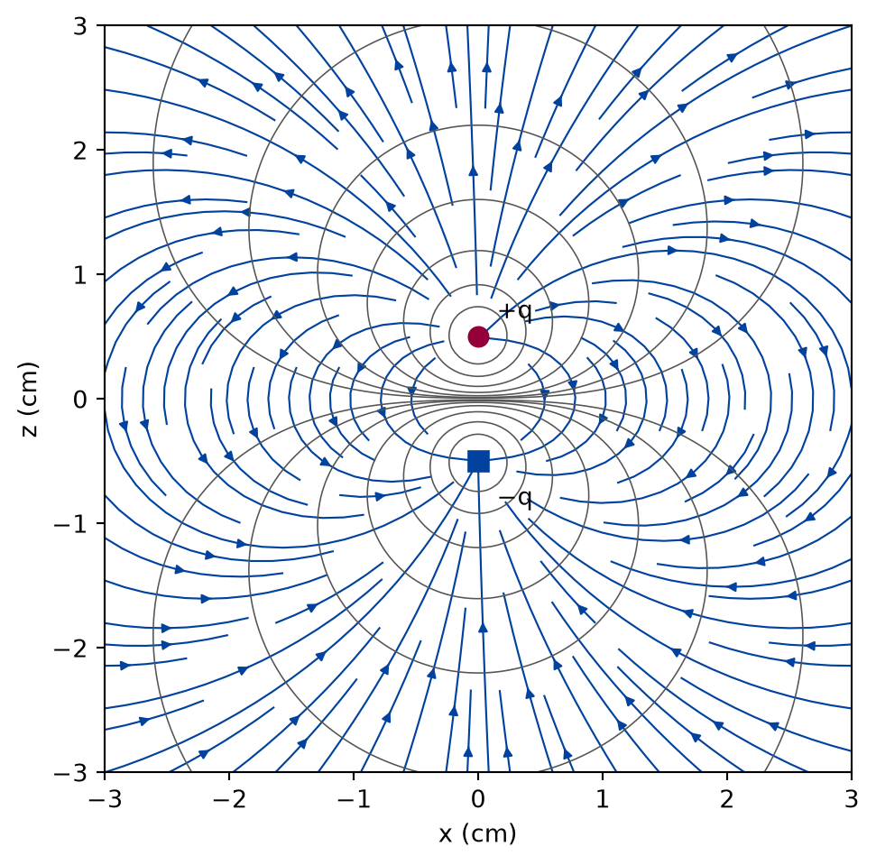
def draw_dipole_field() -> Figure:
    """The field lines and equipotentials of the pair, in a plane through
    both charges, computed by superposition."""
    span = 3.0 * D
    grid_x, grid_z = np.meshgrid(
        np.linspace(-span, span, 161), np.linspace(-span, span, 161)
    )
    plane = np.stack([grid_x, np.zeros_like(grid_x), grid_z], axis=-1)
    # a small shift keeps the grid points off the charges
    plane[..., 0] += 1e-6
    field_plane = coulomb_field(plane, signs, pair)
    potential_plane = coulomb_potential(plane, signs, pair)
    fig, ax = plt.subplots(figsize=(5.6, 5.6))
    ax.streamplot(
        grid_x * 100,
        grid_z * 100,
        field_plane[..., 0],
        field_plane[..., 2],
        color=FIGURE_COLOURS[0],
        density=1.2,
        linewidth=0.8,
        arrowsize=0.8,
    )
    levels = np.sort(
        np.concatenate([-np.geomspace(50, 3000, 7), np.geomspace(50, 3000, 7)])
    )
    ax.contour(
        grid_x * 100,
        grid_z * 100,
        potential_plane,
        levels=levels,
        colors=FIGURE_COLOURS[2],
        linewidths=0.6,
        linestyles="-",
    )
    ax.plot([0.0], [D / 2 * 100], "o", color=FIGURE_COLOURS[1], markersize=8)
    ax.plot([0.0], [-D / 2 * 100], "s", color=FIGURE_COLOURS[0], markersize=8)
    ax.text(0.15, D / 2 * 100 + 0.15, "+q")
    ax.text(0.15, -D / 2 * 100 - 0.35, "\N{MINUS SIGN}q")
    ax.set_aspect("equal")
    ax.set_xlabel("x (cm)")
    ax.set_ylabel("z (cm)")
    return fig

src/pbc/electromagnetism/experiments/electric_fields_and_potential.py, lines 124 to 166, read from the repository when this page was built.

A square plot of the plane through two charges, a positive one above and a negative one below the centre. Blue curved lines run from the upper charge out and around to the lower charge, dense near the charges and spreading out far away. Thin grey closed curves, the equipotentials, surround each charge and cross the field lines at right angles. The pattern is symmetric about the line through both charges. — Figure 1: simulated The field of a pair of opposite charges in a plane through both, computed by superposition. Field lines leave the positive charge and end on the negative one; the equipotentials cross them at right angles, as minus the gradient of the potential must.

The figure shows what the table measures: near the charges the lines are those of two separate charges, and further out the pattern takes the shape of a single dipole. The field is simulated, computed from Coulomb’s law by superposition, and nothing in the drawing uses the dipole formula.

Gauss’s law on a sphere

Four charges, of +1 nC, +2 nC, −0.5 nC, and +3 nC, sit at distances of 0.1 m, 0.22 m, 0.3 m, and 2 m from the origin. The flux of their field out through spheres about the origin is computed for radii that take in more of the charges as they grow.

gauss_charges = np.array([1e-9, 2e-9, -0.5e-9, 3e-9])  # C
gauss_positions = np.array(
    [[0.1, 0.0, 0.0], [0.0, 0.2, 0.09165], [-0.3, 0.0, 0.0], [2.0, 0.0, 0.0]]
)  # m
radii = np.array([0.05, 0.15, 0.25, 0.5, 1.0, 3.0])  # m
GAUSS_TOLERANCE = 1e-8  # a chosen tolerance, relative to the largest charge

src/pbc/electromagnetism/experiments/electric_fields_and_potential.py, lines 49 to 54, read from the repository when this page was built.

def gauss_run(experiment: Experiment) -> None:
    """The flux out through spheres about the origin against the charge
    inside each; record the table."""
    distances = np.linalg.norm(gauss_positions, axis=1)

    def field(p):
        return coulomb_field(p, gauss_charges, gauss_positions)

    rows = []
    worst = 0.0
    for radius in radii:
        inside = float(gauss_charges[distances < radius].sum())
        found = sphere_flux(field, radius=radius, nodes=64) * EPSILON_0
        worst = max(worst, abs(found - inside) / np.max(np.abs(gauss_charges)))
        # A flux of exactly zero can come out as -1e-17 or +1e-17 depending on the
        # CPU's rounding; rounded to the table's four decimals and with the sign
        # of zero removed, both give the same row ("0.0000", never "-0.0000").
        rows.append((radius, inside * 1e9, round(found * 1e9, 4) + 0.0))
    assert worst < GAUSS_TOLERANCE, "the flux does not count the charge inside"

    experiment.table(
        "gauss-run",
        rows,
        [
            ("radius", "m", ".2f"),
            ("charge inside", "nC", ".4f"),
            ("flux times the permittivity", "nC", ".4f"),
        ],
        "The flux of the field of four charges out through a sphere about the "
        "origin, times the vacuum permittivity, against the charge inside the "
        "sphere, for each radius, to four decimals.",
    )

src/pbc/electromagnetism/experiments/electric_fields_and_potential.py, lines 169 to 200, read from the repository when this page was built.

The flux of the field of four charges out through a sphere about the origin, times the vacuum permittivity, against the charge inside the sphere, for each radius, to four decimals.
radius (m)	charge inside (nC)	flux times the permittivity (nC)
0.05	0.0000	0.0000
0.15	1.0000	1.0000
0.25	3.0000	3.0000
0.50	2.5000	2.5000
1.00	2.5000	2.5000
3.00	5.5000	5.5000

Numerically verified (four point charges, spheres that do not pass close to a charge): The flux of the field of point charges out through a sphere is the charge inside divided by $\varepsilon_0$ ; charges outside the sphere add nothing, whatever their distance. At every radius the flux counts exactly the charges inside it: the largest difference is below 1e-08 of the largest charge. The sphere of the smallest radius holds no charge and has no net flux, though the field on it is far from zero; the charge of the last row, at two metres, adds nothing to any sphere smaller than that, and is counted only by the largest. The data are simulated, and the check is Gauss’s law.

Limits

Static charges in vacuum. The lesson computes electrostatics. Moving charges and changing fields need the magnetic field and the full Maxwell equations, which later lessons of the course take up; a material needs its polarisation.
Point charges. A real charge is spread out. Outside a spherical charge the field is that of a point; inside it is not, and the field of an extended body is an integral, not a sum.
A sphere only. Gauss’s law holds for any closed surface. The lesson checks it on spheres, where a simple quadrature is accurate; a charge close to the surface makes the integrand sharp and needs many more nodes than the ones used here.
The numerical gradient has a floor. Below a certain step the round-off of the potential, divided by the step, grows larger than the error of the formula, and the difference stops falling. The steps of the first example stay well above it.

Self-check. A sphere is drawn next to a charge, so that the charge is outside it. What can you say about the field on the sphere and about the flux through it?

The field on the sphere is zero, because no charge is inside.

The field on the sphere is that of the charge outside, and it is not zero. Gauss’s law speaks about the flux, the integral of the outward component, not about the field at each point.
The field is not zero, but the flux through the sphere is zero.

Correct: the field enters the sphere on the side towards the charge and leaves on the far side, and the inward and outward flux cancel exactly.
The flux is small but not zero, and falls as the charge moves further away.

The flux of a charge outside is exactly zero at every distance; the last row of the Gauss example shows a charge outside every sphere but the largest that contributes nothing to them.

Solution to the self-check

The field on the sphere is the field of the charge outside, which is not zero anywhere on it. Its flux is zero: every field line that enters the sphere leaves it again, and the sum of the outward component over the surface cancels. Gauss’s law counts only the charge inside.

Exercises

Exercise 1. On the axis and across it. For the pair of charges of the second example, compare the strength of the field at 0.5 m along the axis of the pair with the strength at the same distance on the plane midway between the charges. What ratio does the dipole formula predict?

Hint 1 of 1 for exercise 1

On the axis, $\hat{\mathbf{n}}$ is parallel to $\mathbf{p}$ ; in the middle plane it is perpendicular to it.

Solution to exercise 1

def axis_and_across() -> tuple[float, float]:
    """Exercise 1: the strength of the field of the pair at 0.5 m on its axis
    and on the plane midway between the charges."""
    on_axis = np.linalg.norm(coulomb_field([[0.0, 0.0, 0.5]], signs, pair))
    across = np.linalg.norm(coulomb_field([[0.5, 0.0, 0.0]], signs, pair))
    return float(on_axis), float(across)

src/pbc/electromagnetism/experiments/electric_fields_and_potential.py, lines 203 to 208, read from the repository when this page was built.

The field on the axis is 1.4383 V/m and the field across it 0.7189 V/m, a ratio of 2.0007. The dipole formula gives $3\,\mathbf{p} - \mathbf{p} = 2\,\mathbf{p}$ on the axis and $-\mathbf{p}$ across it: the field on the axis is twice as strong, and points along the moment, while the field across points against it.

Exercise 2. Where the field vanishes. Charges of +4 nC at the origin and +1 nC at 0.3 m along the axis $x$ . Find the point between them where the field is zero, by computing the field along the line, and check it against the point where the two Coulomb fields have equal strength.

Hint 1 of 1 for exercise 2

At that point the two strengths are equal, so the ratio of the charges is the ratio of the squares of their distances from the point.

Solution to exercise 2

def where_the_field_vanishes() -> tuple[float, float]:
    """Exercise 2: the point between +4 nC and +1 nC, 0.3 m apart, where the
    field computed along the line changes sign, and the point of equal
    strength."""
    line = np.stack(
        [np.linspace(0.01, 0.29, 28_001), np.zeros(28_001), np.zeros(28_001)], axis=1
    )
    along = coulomb_field(line, [4e-9, 1e-9], [[0, 0, 0], [0.3, 0, 0]])[:, 0]
    zero_at = line[np.argmin(np.abs(along)), 0]
    balance = 0.3 * 2.0 / 3.0
    return float(zero_at), balance

src/pbc/electromagnetism/experiments/electric_fields_and_potential.py, lines 211 to 221, read from the repository when this page was built.

The field along the line changes sign at 0.2000 m from the larger charge. Equal strength needs $x/(0.3 - x) = 2$ , the square root of the ratio of the charges, which gives 0.2000 m. The point is closer to the smaller charge, where its weaker field is not yet outweighed.

Exercise 3. A charge close to the sphere. Put a single charge at 0.99 m from the origin and compute the flux through the unit sphere about the origin, with few and with many nodes of the quadrature. Why does it need so many more than the charges of the example?

Hint 1 of 1 for exercise 3

Look at how sharp the field is on the part of the sphere nearest the charge.

Solution to exercise 3

def near_the_sphere(experiment: Experiment) -> list[float]:
    """Exercise 3: the flux through the unit sphere of a charge at 0.99 m,
    for each number of nodes; record the table."""
    near = [[0.99, 0.0, 0.0]]

    def near_field(p):
        return coulomb_field(p, [1e-9], near)

    node_counts = [16, 64, 200, 400, 800]
    near_flux = [
        sphere_flux(near_field, radius=1.0, nodes=n) * EPSILON_0 / 1e-9
        for n in node_counts
    ]
    experiment.table(
        "near-flux",
        list(zip(node_counts, near_flux, strict=True)),
        [
            ("nodes in the polar angle", "", "d"),
            ("flux over the charge over the permittivity", "", ".6f"),
        ],
        "The flux through the unit sphere of a charge just inside it, as a "
        "fraction of the charge over the vacuum permittivity, for each number "
        "of nodes of the quadrature, to six decimals.",
    )
    return near_flux

src/pbc/electromagnetism/experiments/electric_fields_and_potential.py, lines 224 to 248, read from the repository when this page was built.

The flux through the unit sphere of a charge just inside it, as a fraction of the charge over the vacuum permittivity, for each number of nodes of the quadrature, to six decimals.
nodes in the polar angle	flux over the charge over the permittivity
16	0.590017
64	0.824783
200	0.994047
400	0.999980
800	1.000000

With few nodes the flux is far from the charge inside: sixteen nodes in the polar angle give 0.5900 of $q/\varepsilon_0$ . It reaches 1.000000 only with the largest number in the table. A charge a centimetre inside the sphere makes a field that is concentrated in a spot a few centimetres across on the surface, and the rule needs enough nodes to resolve that spot, where the charges of the example are all far from every sphere. The law holds; the quadrature has to see it.

Run this experiment

This page was built from commit 6417e2ff90258bd2d2ba21d217eb7666fd24f680 of the repository.

In a clone at that commit, with the project’s Python packages installed, this command runs the experiment of this page:

uv run --locked --no-dev python -m pbc.electromagnetism.experiments.electric_fields_and_potential results

Files, tests, and every command

The files behind it:

site/lessons/electromagnetism/01-electric-fields-and-potential/index.qmd: this page, with every code cell.
src/pbc/electromagnetism/fields.py: code the experiment runs.
src/pbc/electromagnetism/experiments/electric_fields_and_potential.py: code the experiment runs.
src/pbc/verification/estimates.py: code the experiment runs.
src/pbc/experiment.py: code the experiment runs.
tests/unit/test_electromagnetism.py: tests of that code.
tests/unit/test_electric_fields_and_potential_experiment.py: tests of that code.

With Git and uv installed (see the setup page), run:

git clone https://github.com/taspinar/physics-by-construction.git
cd physics-by-construction
git checkout 6417e2ff90258bd2d2ba21d217eb7666fd24f680
uv sync --locked --no-dev
uv run --locked --no-dev python -m pbc.electromagnetism.experiments.electric_fields_and_potential results

The experiment writes every figure of this page into results/, as <label>.png, and every number and table of the page, as the page shows it, into results/results.json. Its numbers match this page to the digits shown, and its figure files are the ones the page shows; digits beyond those can differ between machines, because floating-point libraries differ. Change the code of the experiment and run it again to see what changes.