Shallow-water equations: still water and the dam break

The depth-averaged balance of mass and momentum for water that is shallow compared with its waves, solved with the shared finite-volume interface; a lake at rest over a bump kept still to round-off, the dam break checked against its exact solution, the depth kept positive over a dry bed, and the budgets of a closed tank.

Course

Fluid dynamics, lesson 4 of 4

Slot

FL5, Shallow-water equations

Methods

Simulation

Difficulty

Advanced, level 3 of 3

What you’ll learn

Derive the shallow-water equations from the conservation of mass and momentum in a column of water, and the speed of their waves
Keep water at rest over an uneven bed exactly still, and explain why a pointwise bed source does not
Check a computed dam break against its exact solution under stated assumptions and a fixed error measure
Keep the depth positive where the water runs onto a dry bed, and check the budgets of a closed tank

Prerequisites

Finite-volume methods and conservation laws.

Before you begin

Calculus: integrals over the depth of a column, and the derivative of an integral whose limits move

Related

none

Previous

Finite-volume methods and conservation laws

Next

An agent runs an experiment

With scripts, this page keeps a record in your browser of whether you completed the lesson. Nothing is stored without them.

With scripts, this place suggests what to do next, with the reason, from the progress saved in your browser. Without them, follow the learning path.

When a dam fails, the water behind it does not fall over all at once. A wall of water runs downstream at a speed set by the depth behind the dam, and a wave of lowering water runs back into the reservoir. Tsunamis crossing an ocean, the tide entering an estuary, and the bore that runs up a river behave the same way. In all of them the water is shallow compared with the length of its waves, and that one fact turns three-dimensional fluid mechanics into two equations for a depth and a velocity.

This lesson derives those equations, the shallow-water equations, and computes them with the finite-volume interface of the previous lesson and a Riemann solver of their own. Two tests are classic. Still water over an uneven bed must stay still; a scheme that sets a lake in motion will invent currents in every computation over real terrain. And a dam break has an exact solution, against which the computed one is measured. Two more follow from the physics: a depth can never be negative, also where water runs onto dry land, and in a closed tank the water’s volume never changes.

Assumptions

Shallow water. The depth is small compared with the length of the waves, so vertical accelerations are negligible and the pressure is hydrostatic, the weight of the water above. Short waves, whose speed depends on their length, are outside the model.
Depth-averaged velocity. The horizontal velocity is the same from the bed to the surface, or is replaced by its average. Friction at the bed, which slows the bottom layer, is not in the model.
One horizontal dimension. The water moves along a channel of unit width; a real flood spreads in two dimensions.
A fixed, frictionless bed. The bed has a height $b(x)$ that does not change, and pushes on the water only through its slope. Erosion and bed friction are not included.
For the dam break: an ideal model. A flat frictionless bed, a dam that vanishes at once, and still water on both sides at the start. The exact solution used as a reference holds under exactly these assumptions; a real dam break has friction, a dam that opens in finite time, and vertical motion at the front.

From a column of water to two equations

Mass

Consider a column of water of unit width above a stretch $[a, c]$ of the bed. With $h(x, t)$ the depth and $u(x, t)$ the depth-averaged velocity, the volume in the column changes only by what flows through its two vertical sides, $h u$ at each:

$\frac{\mathrm{d}}{\mathrm{d}t}\int_a^c h\,\mathrm{d}x = (h u)\big|_a - (h u)\big|_c \quad\Longrightarrow\quad \frac{\partial h}{\partial t} + \frac{\partial (h u)}{\partial x} = 0 .$

Momentum

The momentum of the column, per unit density, is $\int h u\,\mathrm{d}x$ . It changes by the momentum carried through the sides, $h u^2$ , by the pressure on the sides, and by the push of a sloping bed. The pressure is hydrostatic, $\rho g$ times the depth below the surface, so its integral over a side of depth $h$ is $\rho g h^2/2$ . The bed, sloping by $b_x$ , pushes on the column with the horizontal force $-\rho g h\,b_x$ per unit length. Divided by the density,

$\frac{\partial (h u)}{\partial t} + \frac{\partial}{\partial x}\!\left(h u^2 + \frac{g h^2}{2}\right) = -g h\,\frac{\partial b}{\partial x} .$

Over a flat bed this is a conservation law for $q = (h, hu)$ with the flux $f(q) = (hu,\ hu^2 + g h^2/2)$ , the system that the previous lesson put into the shared interface. Over a sloping bed the momentum has a source.

Waves

Small disturbances of still water of depth $h_0$ satisfy, to first order, $h_t + h_0 u_x = 0$ and $u_t + g h_x = 0$ , which combine into the wave equation with the speed

$c = \sqrt{g h_0} .$

Long waves in shallow water travel at a speed set by the depth alone: a tsunami over an ocean four kilometres deep moves at the speed of an aircraft, and slows as it reaches the coast. In a flow of velocity $u$ the two waves move at $u - c$ and $u + c$ ; the CFL condition limits the step by the larger of $|u| + c$ .

Water at rest over a bump

For still water, $u = 0$ , with a flat surface $h + b = \text{const}$ , the two sides of the momentum equation are each non-zero and cancel exactly: the pressure gradient $\partial_x(g h^2/2) = g h\,h_x$ equals $-g h\,b_x$ . A scheme that approximates the flux difference and the source independently makes two errors of order $\Delta x$ that do not cancel, and the lake starts to move. Hydrostatic reconstruction, introduced by Audusse and co-authors, rebuilds the depth on each side of a face over the higher of the two beds, $h^* = \max(0,\ h + b - \max(b_L, b_R))$ , takes the flux between the rebuilt states, and adds to each cell the pressure difference $g(h^2 - h^{*2})/2$ at its faces as the source. For a lake at rest the rebuilt states on the two sides of a face are equal, and the source cancels the flux difference to the last bit. The scheme is called well balanced. Its mass update is still a difference of fluxes, so the water’s volume is conserved.

The dam break

Still water of depth $h_u$ left of $x = 0$ and $h_d < h_u$ right of it, over a flat bed, with the dam removed at $t = 0$ . The exact solution, a Riemann problem of the system, has two waves:

a rarefaction running into the deep water, from $x = -c_u t$ , in which $u + 2c$ keeps its upstream value $2c_u$ and the depth falls as $h = (2c_u - x/t)^2/(9g)$ ;
a shock, the front, running into the shallow water. Mass and momentum conserved across it give the middle depth $h_m$ as the root of $2\left(c_u - \sqrt{g h_m}\right) = (h_m - h_d)\sqrt{\frac{g\,(h_m + h_d)}{2 h_m h_d}},$ the velocity $u_m$ behind both waves, and the front speed $s = h_m u_m/(h_m - h_d)$ .

Over a dry bed, $h_d = 0$ , there is no shock: the rarefaction reaches all the way to a front at $x = 2c_u t$ , where the depth goes to zero.

The comparison, fixed in advance. One-dimensional ideal shallow water over a flat frictionless bed, $g = 9.81\ \mathrm{m/s^2}$ ; still water of depth $2$ m left of the dam at $x = 0$ and $0.5$ m right of it, on a domain from $-10$ to $10$ m with open ends; the time $t = 1$ s, before any wave reaches an end. The reference is the exact solution above. The error measures are the integral over the domain of the absolute difference of the depths, and the position of the front, taken where the computed depth crosses the mean of $h_m$ and $h_d$ , against the exact front $s\,t$ , in cell widths.

The Riemann solver and the depth

The HLL flux of the previous lesson needs the speeds of the slowest and fastest waves of a face. With the estimates of Einfeldt, the smallest and largest of $u - c$ and $u + c$ of the two states and of their Roe average, the scheme keeps every depth non-negative under the CFL condition, also where one side of a face is dry. A dry cell has no velocity; the program sets it to zero below a depth of $10^{-10}$ m.

Code

The physical flux, the HLL Riemann solver, the reflecting walls, and the well-balanced bed are the shallow-water parts; the update, the steps, and the budgets are those of the shared finite-volume interface.

def flux(q: Array) -> Array:
    """The physical flux (h u, h u^2 + g h^2 / 2) of the states ``q``."""
    h = q[..., 0]
    u = velocity(q)
    return np.stack([h * u, h * u * u + 0.5 * GRAVITY * h * h], axis=-1)

src/pbc/fluids/shallow_water.py, lines 55 to 59, read from the repository when this page was built.

def well_balanced(
    bed: Array, dx: float, boundary: Boundary
) -> tuple[Callable[[Array], Array], Callable[[Array], Array]]:
    """The face fluxes and the bed source of hydrostatic reconstruction over
    the cell bed heights ``bed`` (m) on cells of width ``dx`` (m), for
    ``finite_volume.evolve``.

    At each face the two depths are rebuilt over the higher of the two beds,
    h* = max(0, h + b - max(b_left, b_right)), keeping each cell's velocity,
    and the HLL flux is taken between the rebuilt states. The source adds to
    each cell the pressure g / 2 (h^2 - h*^2) of the difference at its two
    faces. For water at rest with a flat surface the rebuilt states on the two
    sides of a face are equal, the fluxes are the pressure g h*^2 / 2, and
    the source cancels their difference exactly."""
    bed_padded = np.concatenate([[bed[0]], bed, [bed[-1]]])
    top = np.maximum(bed_padded[:-1], bed_padded[1:])

    def rebuilt(q: Array) -> tuple[Array, Array, Array]:
        padded = with_ghosts(q, boundary)
        h, u = padded[:, 0], velocity(padded)
        h_left = np.maximum(0.0, h[:-1] + bed_padded[:-1] - top)
        h_right = np.maximum(0.0, h[1:] + bed_padded[1:] - top)
        left = np.stack([h_left, h_left * u[:-1]], axis=-1)
        right = np.stack([h_right, h_right * u[1:]], axis=-1)
        return left, right, h

    def fluxes(q: Array) -> Array:
        left, right, _ = rebuilt(q)
        return hll_flux(left, right)

    def source(q: Array) -> Array:
        left, right, h = rebuilt(q)
        cell = h[1:-1]
        # The cell's own side of its right face is left[1:], of its left face
        # right[:-1].
        push = 0.5 * GRAVITY * (left[1:, 0] ** 2 - right[:-1, 0] ** 2)
        return np.stack([np.zeros_like(cell), push], axis=-1) / dx

    return fluxes, source

src/pbc/fluids/shallow_water.py, lines 103 to 141, read from the repository when this page was built.

def pointwise_source(
    bed: Array, dx: float, boundary: Boundary
) -> tuple[Callable[[Array], Array], Callable[[Array], Array]]:
    """The naive discretisation over the bed ``bed`` (m): HLL fluxes between
    the cell states as they are, and the source -g h db/dx with a central
    difference of the bed. Each is consistent, but their errors do not cancel
    for water at rest, which then starts to move."""
    bed_padded = np.concatenate([[bed[0]], bed, [bed[-1]]])
    slope = (bed_padded[2:] - bed_padded[:-2]) / (2.0 * dx)

    def fluxes(q: Array) -> Array:
        return interface_fluxes(q, hll_flux, boundary)

    def source(q: Array) -> Array:
        return np.stack([np.zeros(len(q)), -GRAVITY * q[:, 0] * slope], axis=-1)

    return fluxes, source

src/pbc/fluids/shallow_water.py, lines 144 to 160, read from the repository when this page was built.

def dam_break(upstream: float, downstream: float) -> DamBreak:
    """The exact solution of the dam break: a rarefaction into the deep water
    and, over a wet bed, a shock into the shallow water.

    The middle depth h_m is the root of 2 (c_up - c_m) = (h_m - h_d)
    sqrt(g (h_m + h_d) / (2 h_m h_d)), the velocity behind the rarefaction
    equal to the velocity behind the shock, with c = sqrt(g h); the shock
    moves at h_m u_m / (h_m - h_d), which conserves the mass across it."""
    if not upstream > downstream >= 0:
        raise ValueError("the dam holds deeper water upstream")
    c_up = np.sqrt(GRAVITY * upstream)
    if downstream == 0:
        return DamBreak(upstream, 0.0, 0.0, 2.0 * c_up, 2.0 * c_up)

    def mismatch(h: float) -> float:
        behind_fan = 2.0 * (c_up - np.sqrt(GRAVITY * h))
        behind_shock = (h - downstream) * np.sqrt(
            0.5 * GRAVITY * (h + downstream) / (h * downstream)
        )
        return behind_fan - behind_shock

    middle = brentq(mismatch, downstream, upstream, xtol=1e-15, rtol=1e-15)
    u_middle = 2.0 * (c_up - np.sqrt(GRAVITY * middle))
    return DamBreak(
        upstream,
        downstream,
        middle,
        u_middle,
        middle * u_middle / (middle - downstream),
    )

src/pbc/fluids/shallow_water.py, lines 203 to 232, read from the repository when this page was built.

Worked examples

A lake at rest

A lake with a flat surface one metre above the datum, over a bed with a smooth bump of half a metre, between two walls ten metres apart. The water is at rest and must stay so. It is run for five seconds, long enough for a wave to cross the lake several times, once with hydrostatic reconstruction and once with the pointwise bed source.

LAKE_LENGTH = 10.0  # m, from -5 to 5, walls at both ends
SURFACE = 1.0  # m above the datum
BUMP = 0.5  # m, the height of the bed's bump, 0.5 exp(-x^2)
LAKE_TIME = 5.0  # s
lake_cells = [50, 100, 200, 400]
STILL_BOUND = 1e-12  # m/s and m

src/pbc/fluids/experiments/shallow_water_equations.py, lines 43 to 48, read from the repository when this page was built.

def lake_run(experiment: Experiment) -> tuple[float, float]:
    """The lake at rest run with the two treatments of the bed, for each
    grid; record the table and return the order of the spurious speed of the
    pointwise source and that speed on the coarsest grid."""
    rows, spurious = [], []
    for n in lake_cells:
        bed, water, dx = lake(n)
        fluxes, source = well_balanced(bed, dx, reflective)
        kept = evolve(water, dx, LAKE_TIME, fluxes, max_speed, COURANT, source).q
        fluxes, source = pointwise_source(bed, dx, reflective)
        moved = evolve(water, dx, LAKE_TIME, fluxes, max_speed, COURANT, source).q
        speed = float(np.max(np.abs(velocity(kept))))
        level = float(np.max(np.abs(kept[:, 0] + bed - SURFACE)))
        assert speed < STILL_BOUND and level < STILL_BOUND, "the lake moved"
        spurious.append(float(np.max(np.abs(velocity(moved)))))
        rows.append(
            (n, f"below {STILL_BOUND:.0e}", spurious[-1],
             float(np.max(np.abs(moved[:, 0] + bed - SURFACE))))
        )  # fmt: skip
    order = fitted_order(LAKE_LENGTH / np.array(lake_cells), spurious)
    assert order > 0.9, "the spurious current does not fall with the cell width"
    experiment.table(
        "lake-run",
        rows,
        [
            ("cells", "", "d"),
            ("largest speed, reconstruction", "m/s", ""),
            ("largest speed, pointwise source", "m/s", ".2e"),
            ("largest surface change, pointwise source", "m", ".2e"),
        ],
        "Still water with a flat surface over a bump of the bed, after five "
        "seconds, for each grid: the largest speed with hydrostatic "
        "reconstruction (where the surface also stays within the same bound), "
        "and the largest speed and change of the surface with the pointwise "
        "bed source.",
    )
    return order, spurious[0]

src/pbc/fluids/experiments/shallow_water_equations.py, lines 81 to 117, read from the repository when this page was built.

Still water with a flat surface over a bump of the bed, after five seconds, for each grid: the largest speed with hydrostatic reconstruction (where the surface also stays within the same bound), and the largest speed and change of the surface with the pointwise bed source.
cells	largest speed, reconstruction (m/s)	largest speed, pointwise source (m/s)	largest surface change, pointwise source (m)
50	below 1e-12	1.56e-01	6.92e-03
100	below 1e-12	7.89e-02	3.97e-03
200	below 1e-12	3.95e-02	2.18e-03
400	below 1e-12	1.97e-02	1.24e-03

Numerically verified (the lake and bump of the example, HLL flux, walls at both ends, five seconds): With hydrostatic reconstruction a lake at rest over an uneven bed stays at rest to round-off; with a pointwise bed source it starts to move, with a speed that falls only in proportion to the cell width. The reconstruction keeps every speed and the surface within 1e-12. The pointwise source drives currents of up to 0.156 m/s on the coarsest grid, in water that should not move; the fitted order is 1.00. Over real terrain, with bumps everywhere, such currents would be indistinguishable from the flow the model is meant to compute.

The dam break against its exact solution

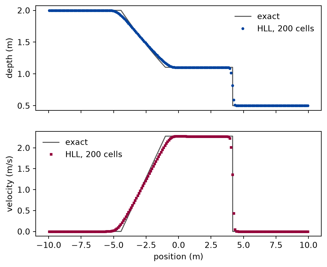
The comparison fixed in the explanation, on grids from one hundred to sixteen hundred cells. The exact solution has a middle depth of 1.1035 m and a velocity of 2.2785 m/s between the waves, and a front that moves at 4.1663 m/s.

LENGTH = 20.0  # m, from -10 to 10, open ends
UPSTREAM = 2.0  # m, still water left of the dam at x = 0
DOWNSTREAM = 0.5  # m, still water right of it
DAM_TIME = 1.0  # s
dam_cells = [100, 200, 400, 800, 1600]

src/pbc/fluids/experiments/shallow_water_equations.py, lines 52 to 56, read from the repository when this page was built.

def dam_run(experiment: Experiment) -> float:
    """The wet dam break against the exact solution, for each grid: the
    integral of the absolute depth error and the position of the front;
    record the table and return the order of the depth error."""
    exact = dam_break(UPSTREAM, DOWNSTREAM)
    front = exact.front_speed * DAM_TIME
    level = 0.5 * (exact.middle + DOWNSTREAM)
    rows, errors = [], []
    for n in dam_cells:
        x, q = dam_profile(n)
        dx = LENGTH / n
        errors.append(float(np.sum(np.abs(q[:, 0] - exact.depth(x, DAM_TIME))) * dx))
        found = front_position(q[:, 0], x, level)
        assert abs(found - front) < dx, "the front is more than a cell off"
        rows.append((n, dx, errors[-1], found, abs(found - front) / dx))
    order = fitted_order(LENGTH / np.array(dam_cells), errors)
    assert order > 0.7, "the dam break does not converge"
    experiment.table(
        "dam-run",
        rows,
        [
            ("cells", "", "d"),
            ("cell width", "m", ".4f"),
            ("depth error", "m²", ".3e"),
            ("front", "m", ".4f"),
            ("front error", "cells", ".2f"),
        ],
        "The dam break over a wet bed after one second, for each grid: the "
        "integral over the domain of the absolute difference between the "
        "computed and the exact depth, the computed position of the front, "
        "and its distance from the exact front in cell widths.",
    )
    return order

src/pbc/fluids/experiments/shallow_water_equations.py, lines 141 to 173, read from the repository when this page was built.

The dam break over a wet bed after one second, for each grid: the integral over the domain of the absolute difference between the computed and the exact depth, the computed position of the front, and its distance from the exact front in cell widths.
cells	cell width (m)	depth error (m²)	front (m)	front error (cells)
100	0.2000	3.465e-01	4.1607	0.03
200	0.1000	2.021e-01	4.1571	0.09
400	0.0500	1.118e-01	4.1565	0.20
800	0.0250	6.553e-02	4.1599	0.26
1600	0.0125	3.549e-02	4.1620	0.35

Numerically verified (one-dimensional ideal shallow water, flat frictionless bed, the depths, domain, and time of the comparison, HLL flux): The computed dam break converges to the exact solution of the ideal model: the integrated depth error falls with an order near one, and the front lies within one cell of the exact front on every grid. The fitted order of the depth error is 0.82, a little below one: the error is largest at the corners of the rarefaction, where the first-order scheme rounds the kinks, as the fan of the Burgers lesson showed. The front is captured within a fraction of a cell; its speed comes out of the conservative fluxes, which is the Rankine-Hugoniot condition of the system.

def draw_dam_break() -> Figure:
    """The depth and the velocity of the wet dam break after one second on
    two hundred cells, against the exact solution."""
    n = 200
    x, q = dam_profile(n)
    exact = dam_break(UPSTREAM, DOWNSTREAM)
    fine = np.linspace(-LENGTH / 2, LENGTH / 2, 4001)
    fig, (top, bottom) = plt.subplots(2, 1, figsize=(6.4, 5.2), sharex=True)
    top.plot(
        fine,
        exact.depth(fine, DAM_TIME),
        color=FIGURE_COLOURS[2],
        linewidth=1.2,
        label="exact",
    )
    top.plot(
        x,
        q[:, 0],
        color=FIGURE_COLOURS[0],
        linestyle="none",
        marker="o",
        markersize=2.5,
        label="HLL, 200 cells",
    )
    top.set_ylabel("depth (m)")
    top.legend(loc="upper right", frameon=False)
    bottom.plot(
        fine,
        exact.velocity(fine, DAM_TIME),
        color=FIGURE_COLOURS[2],
        linewidth=1.2,
        label="exact",
    )
    bottom.plot(
        x,
        velocity(q),
        color=FIGURE_COLOURS[1],
        linestyle="none",
        marker="s",
        markersize=2.5,
        label="HLL, 200 cells",
    )
    bottom.set_ylabel("velocity (m/s)")
    bottom.set_xlabel("position (m)")
    bottom.legend(loc="upper left", frameon=False)
    return fig

src/pbc/fluids/experiments/shallow_water_equations.py, lines 176 to 221, read from the repository when this page was built.

Two plots sharing a position axis. Top: depth against position. The exact depth is flat and high on the left, falls along a straight-sided ramp, is flat at a middle level, and drops in a vertical step to the low level on the right. The computed points follow it, with rounded corners at the ends of the ramp and a step one or two points wide. Bottom: velocity against position. The exact velocity is zero on the left, rises linearly across the ramp, is constant in the middle, and drops to zero at the front. The computed points follow it in the same way. — Figure 1: simulated The dam break after one second: the computed depth and velocity follow the exact solution, a rarefaction into the deep water and a front into the shallow water, rounded at the corners of the rarefaction and sharp at the front.

The figure shows both waves of the Riemann problem. The data are simulated on two hundred cells, and the reference is the exact solution of the ideal model, which says nothing about friction or the vertical motion at a real front.

Water onto a dry bed

The dam now holds one metre of water, and the bed beyond it is dry. The exact front runs at $2c_u$ , reaching 6.264 m after one second. The program steps the solution itself, to see the depth of every cell at every step.

DRY_UPSTREAM = 1.0  # m, nothing right of the dam
dry_cells = [200, 400, 800, 1600]
WET = 1e-3  # m: the front is the last cell deeper than this

src/pbc/fluids/experiments/shallow_water_equations.py, lines 60 to 62, read from the repository when this page was built.

def dry_run(experiment: Experiment) -> float:
    """The dam break over a dry bed, step by step, for each grid: the
    smallest depth of any cell at any step, the depth error, and the wet
    front against the exact front 2 sqrt(g h) t; record the table and return
    the smallest depth of all runs."""
    exact = dam_break(DRY_UPSTREAM, 0.0)
    rows = []
    lowest = np.inf
    for n in dry_cells:
        dx = LENGTH / n
        x = centres(n, LENGTH)
        q = np.stack([np.where(x < 0, DRY_UPSTREAM, 0.0), np.zeros(n)], axis=-1)
        t, smallest = 0.0, 0.0
        while t < DAM_TIME:
            dt = min(COURANT * dx / max_speed(q), DAM_TIME - t)
            q = conservative_update(
                q, interface_fluxes(q, hll_flux, transmissive), dt, dx
            )
            smallest = min(smallest, float(np.min(q[:, 0])))
            t = DAM_TIME if t + dt >= DAM_TIME else t + dt
        lowest = min(lowest, smallest)
        error = float(np.sum(np.abs(q[:, 0] - exact.depth(x, DAM_TIME))) * dx)
        rows.append((n, smallest, error, float(x[q[:, 0] > WET].max())))
    assert lowest >= 0.0, "a depth became negative"
    experiment.table(
        "dry-run",
        rows,
        [
            ("cells", "", "d"),
            ("smallest depth at any step", "m", ".1f"),
            ("depth error", "m²", ".3e"),
            ("last cell deeper than a millimetre", "m", ".3f"),
        ],
        "The dam break over a dry bed after one second, for each grid: the "
        "smallest depth of any cell at any step, the integral over the domain "
        "of the absolute depth error, and the centre of the last cell whose "
        "depth exceeds one millimetre.",
    )
    return lowest

src/pbc/fluids/experiments/shallow_water_equations.py, lines 224 to 262, read from the repository when this page was built.

The dam break over a dry bed after one second, for each grid: the smallest depth of any cell at any step, the integral over the domain of the absolute depth error, and the centre of the last cell whose depth exceeds one millimetre.
cells	depth error (m²)	last cell deeper than a millimetre (m)
200	1.124e-01	4.850
400	6.696e-02	5.075
800	4.009e-02	5.312
1600	2.376e-02	5.506

Numerically verified (the dry dam break of the example, four grids, Courant number nine tenths): With the HLL flux and Einfeldt’s wave speeds under the CFL condition, no depth becomes negative at any step of the dry dam break, and the depth error falls as the grid is refined. The smallest depth of any cell at any step is zero, on the dry bed, and never below. The wet front, the last cell deeper than a millimetre, lags behind the exact front: near the tip the exact depth falls as the square of the distance to it, so the last metre of the rarefaction is a film thinner than the threshold, and a first-order scheme spreads that film over many cells. The lag shrinks with the cell width, slowly.

Limits

The exact solution is of the model. The dam-break reference is exact for ideal one-dimensional shallow water over a flat frictionless bed. It is not a measured dam break; real fronts are slowed by friction and are not vertical.
Hydrostatic pressure. The model has no dispersion: all long waves travel at $\sqrt{g h}$ . Waves shorter than a few depths travel slower in reality, and a real bore breaks into undulations that the model cannot show.
Lake at rest only. Hydrostatic reconstruction keeps water at rest still. A steady flow over a bump, which moves but does not change, is not kept exactly by it.
Dry fronts converge slowly. Positivity is guaranteed, accuracy at a wet and dry boundary is not; the front of the dry run lags on every grid of the table.
One dimension. A flood, a tsunami, or a tide spreads in two horizontal dimensions; the method extends face by face, which the capstone of the course does.

Self-check. A model of a harbour over an uneven seabed, started from still water and run with no wind, tide, or waves, shows currents of a few centimetres per second after an hour. What is the most likely cause?

The shallow-water equations predict slow currents over an uneven bed even without forcing.

Still water with a flat surface is an exact solution of the equations over any bed: the pressure gradient and the bed slope cancel. The currents are not in the model.
The scheme is not well balanced: its flux differences and its bed source do not cancel for water at rest.

Correct: a pointwise bed source leaves an error of order of the cell width, which drives currents that look like flow, as the lake example measured.
Round-off accumulates over the many steps of an hour.

Round-off stays at its level; the well-balanced run of the lake example kept the speeds below its bound over many crossings.

Solution to the self-check

The scheme. Still water over any bed is an exact solution of the shallow-water equations, and a well-balanced scheme keeps it to round-off. A scheme that discretises the pressure flux and the bed source independently leaves an error of order of the cell width that drives currents, which shrink as the grid is refined; refining the grid is the test that tells them apart from physics.

Exercises

Exercise 1. The speed of a long wave. Put a small hump of water, $1$ mm high and about $1$ m wide, on still water $1$ m deep. It splits into two waves running apart. Measure the speed of the right-going wave from the position of its crest at two times, and compare it with $\sqrt{g h}$ .

Hint 1 of 1 for exercise 1

Take the two times after the waves have separated, and far apart.

Solution to exercise 1

def wave_speed() -> tuple[float, float]:
    """Exercise 1: a small hump on still water one metre deep splits into two
    waves; the speed of the right-going one from its crest at two times, and
    sqrt(g h)."""
    n, depth = 2000, 1.0
    dx = LENGTH / n
    x = centres(n, LENGTH)
    q = np.stack([depth + 0.001 * np.exp(-((x / 0.5) ** 2)), np.zeros(n)], axis=-1)

    def fluxes(state):
        return interface_fluxes(state, hll_flux, transmissive)

    first = evolve(q, dx, 0.5, fluxes, max_speed, COURANT).q
    second = evolve(first, dx, 1.0, fluxes, max_speed, COURANT).q
    right = x > 0
    crests = [x[right][np.argmax(s[right, 0])] for s in (first, second)]
    return float((crests[1] - crests[0]) / 1.0), float(np.sqrt(GRAVITY * depth))

src/pbc/fluids/experiments/shallow_water_equations.py, lines 265 to 281, read from the repository when this page was built.

The crest moves at 3.140 m/s, against $\sqrt{g h} =$ 3.132 m/s. The difference is within a cell width per second, the resolution of a crest found at a cell centre, plus the slight extra speed of a wave of finite height, which travels on water a little deeper than the rest.

Exercise 2. A closed tank. Run the dam break of the second example between two walls for $10$ s, while the waves reflect back and forth. Is the volume of the water conserved? Is its momentum?

Hint 1 of 1 for exercise 2

The walls let no water through, but the water presses on them.

Solution to exercise 2

def tank_run(experiment: Experiment) -> None:
    """Exercise 2: the wet dam break between two walls for ten seconds;
    record the change of the mass and of the momentum and the largest
    residual of their budgets."""
    n = 400
    dx = LENGTH / n
    x = centres(n, LENGTH)
    water = np.stack([np.where(x < 0, UPSTREAM, DOWNSTREAM), np.zeros(n)], axis=-1)
    run = evolve(
        water,
        dx,
        10.0,
        lambda q: interface_fluxes(q, hll_flux, reflective),
        max_speed,
        COURANT,
    )
    residual = np.max(np.abs(run.budget_residual), axis=0)
    scale = np.abs(run.totals[0]) + 1.0
    assert np.all(residual / scale < TANK_BOUND), "a budget of the tank did not close"
    # Rounded to the table's four decimals with the sign of zero removed.
    change = np.round(run.totals[-1] - run.totals[0], 4) + 0.0
    bound = f"below {TANK_BOUND:.0e}"
    experiment.table(
        "tank-run",
        [
            ("water volume per width", "m²", change[0], bound),
            ("momentum per density and width", "m³/s", change[1], bound),
        ],
        [
            ("quantity", "", ""),
            ("unit", "", ""),
            ("change after ten seconds", "", ".4f"),
            ("largest budget residual", "", ""),
        ],
        "The dam break in a tank with walls at both ends, for ten seconds on "
        "four hundred cells: the change of each total, and the largest "
        "difference over all steps between that change and what crossed the "
        "walls, relative to the total at the start plus one.",
    )

src/pbc/fluids/experiments/shallow_water_equations.py, lines 284 to 322, read from the repository when this page was built.

The dam break in a tank with walls at both ends, for ten seconds on four hundred cells: the change of each total, and the largest difference over all steps between that change and what crossed the walls, relative to the total at the start plus one.
quantity	unit	change after ten seconds	largest budget residual
water volume per width	m²	0.0000	below 1e-13
momentum per density and width	m³/s	-14.8635	below 1e-13

The volume does not change: the mass flux through a wall, computed from the water and its mirror image, is exactly zero. The momentum changes, because the walls push on the water with the pressure of the water against them, and the budget accounts for it to round-off. The water sloshes, and its total momentum swings with it.

Run this experiment

This page was built from commit 3a83ab640162bf2b624c2b254d917ed5bdc7090d of the repository.

In a clone at that commit, with the project’s Python packages installed, this command runs the experiment of this page:

uv run --locked --no-dev python -m pbc.fluids.experiments.shallow_water_equations results

Files, tests, and every command

The files behind it:

site/lessons/fluids/04-shallow-water-equations/index.qmd: this page, with every code cell.
src/pbc/fluids/shallow_water.py: code the experiment runs.
src/pbc/fluids/finite_volume.py: code the experiment runs.
src/pbc/fluids/experiments/shallow_water_equations.py: code the experiment runs.
src/pbc/verification/estimates.py: code the experiment runs.
src/pbc/experiment.py: code the experiment runs.
tests/unit/test_fluids.py: tests of that code.
tests/unit/test_shallow_water_equations_experiment.py: tests of that code.

With Git and uv installed (see the setup page), run:

git clone https://github.com/taspinar/physics-by-construction.git
cd physics-by-construction
git checkout 3a83ab640162bf2b624c2b254d917ed5bdc7090d
uv sync --locked --no-dev
uv run --locked --no-dev python -m pbc.fluids.experiments.shallow_water_equations results

The experiment writes every figure of this page into results/, as <label>.png, and every number and table of the page, as the page shows it, into results/results.json. Its numbers match this page to the digits shown, and its figure files are the ones the page shows; digits beyond those can differ between machines, because floating-point libraries differ. Change the code of the experiment and run it again to see what changes.