Kinematics as a program

Motion along a line under a known acceleration, written as a state and an update rule, and checked against the exact solution.

Course

Classical mechanics, lesson 1 of 28

Slot

M1, Kinematics as a program

Methods

Simulation

Difficulty

Introductory, level 1 of 3

What you’ll learn

• Write motion along a line as a state and an update rule
• Check a simulation against the exact solution for constant acceleration
• Measure how the error of Euler stepping shrinks with the time step

Prerequisites

none on this site.

Before you begin

• Calculus: derivatives, integrals, and Taylor expansion to second order
• Python: functions, dataclasses, and NumPy arrays
• Logarithms: the base-2 logarithm, and reading a log-log plot

Related

Proving what the simulation showed

Previous

none; this is the first lesson of the learning path

Next

Newton’s laws as a first-order system

With scripts, this page keeps a record in your browser of whether you completed the lesson. Nothing is stored without them.

With scripts, this place suggests what to do next, with the reason, from the progress saved in your browser. Without them, follow the learning path.

Where is a thrown ball one second after it leaves the hand, when all we know is how fast it started and how its speed changes? The same question is asked of a braking car, a rocket under thrust, and a spacecraft on approach, and almost none of them has a formula for the answer. What they share is a rule for how the motion changes from one instant to the next, and a program can follow such a rule.

Kinematics describes motion without asking what causes it. The acceleration $a(t)$ is given, and the task is to find the velocity $v(t)$ and the position $x(t)$. This lesson turns that task into a program: it holds a state, advances the state by a small time step, and repeats. The method is explicit Euler, the simplest one there is.

Because the acceleration is known, the exact motion is known too. So we can measure how wrong the program is, and how the error shrinks when the time step does. Checking a simulation against something you can calculate by hand is the habit the rest of this course builds on.

Assumptions

The model and the program rest on these assumptions. Each one names what goes wrong when it does not hold.

1. A point particle on a line. One number $x(t)$ gives the position. A body that rotates, bends, or moves in a plane needs more state than this lesson carries.
2. The acceleration depends on time only. $a(t)$ is known in advance and does not depend on where the particle is or how fast it moves. A spring (acceleration depends on $x$) or air drag (depends on $v$) breaks this. The update rule below still runs for them, but the exact solutions used here for comparison no longer apply.
3. Newtonian motion. Speeds are far below the speed of light, and one clock serves everyone.
4. The acceleration is smooth within a step. The error estimate needs $a(t)$ to change little during one time step. A jump inside a step, such as an impact, makes the error larger than estimated.
5. Round-off is negligible. The program computes with double-precision floating-point numbers, and every operation rounds its result. For the time steps used here that rounding is many orders of magnitude smaller than the error of the method. With very many very small steps it would become visible.

The worked examples add one more: free fall without air. Near the Earth’s surface and without drag the acceleration is the constant $-g$. For a light ball at high speed, drag is not small, and a later lesson adds it.

From rates of change to an update rule

Velocity is the rate of change of position, and acceleration is the rate of change of velocity:

$$\frac{\mathrm{d}x}{\mathrm{d}t} = v, \qquad \frac{\mathrm{d}v}{\mathrm{d}t} = a(t).$$

Everything the program needs to know at one instant is the triple $(t, x, v)$. That triple is the state.

Over a short time $\Delta t$ the Taylor expansions of position and velocity are

$$\begin{aligned} x(t + \Delta t) &= x(t) + v(t)\,\Delta t + \tfrac{1}{2}\,a(t)\,\Delta t^{2} + \dots \\ v(t + \Delta t) &= v(t) + a(t)\,\Delta t + \dots \end{aligned}$$

Explicit Euler keeps the terms that are linear in $\Delta t$ and drops the rest. Writing $x_n$ and $v_n$ for the computed values at time $t_n = t_0 + n\,\Delta t$, the update rule is

$$\begin{aligned} x_{n+1} &= x_n + v_n\,\Delta t, \\ v_{n+1} &= v_n + a(t_n)\,\Delta t, \\ t_{n+1} &= t_n + \Delta t. \end{aligned}$$

The right-hand sides use only values the program already has, which is what “explicit” means.

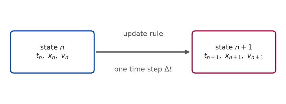
def draw_state_and_update() -> Figure:
    """The state and the update rule, as a sketch."""
    fig, ax = canvas(6.4, 2.2, (0, 10), (0, 3.4))
    state_box(ax, (1.7, 1.7), "state $n$\n" r"$t_n,\ x_n,\ v_n$", width=3.0, height=1.5)
    state_box(
        ax,
        (8.3, 1.7),
        "state $n+1$\n" r"$t_{n+1},\ x_{n+1},\ v_{n+1}$",
        width=3.0,
        height=1.5,
        colour=1,
    )
    arrow(ax, (3.3, 1.7), (6.7, 1.7), colour=2)
    text(ax, (5.0, 2.35), "update rule", colour=2)
    text(ax, (5.0, 1.05), r"one time step $\Delta t$", colour=2)
    return fig

src/pbc/mechanics/experiments/kinematics.py, lines 56 to 71, read from the repository when this page was built.

Figure 1: conceptual The program holds one state and one rule. The rule turns the state at one step into the state at the next, using nothing but that state.

A simulation is this arrow applied again and again, and everything the arrow may use sits in the box on its left. The sketch computes nothing.

How large is the error?

One step drops terms of size $\Delta t^{2}$, so a step adds an error of at most $C\,\Delta t^{2}$ for some constant $C$ that depends on how fast $a(t)$ changes. Reaching a fixed time $T$ takes $T / \Delta t$ steps, and the dropped terms add up to at most $(T / \Delta t)\,C\,\Delta t^{2} = C\,T\,\Delta t$: an error of size $\Delta t$. This bound is an argument for the order, not yet a measurement; the examples measure it. Explicit Euler is a first-order method: halve the time step and the error at time $T$ halves, at twice the work.

For a constant acceleration $a$ we can say exactly what the method does. The exact motion from the initial values $x_0$ and $v_0$ at $t_0 = 0$ is

$$x(t) = x_0 + v_0\,t + \tfrac{1}{2}\,a\,t^{2}, \qquad v(t) = v_0 + a\,t.$$

The update rule adds $a\,\Delta t$ to the velocity in every step, so $v_n = v_0 + a\,t_n$: the computed velocity is exact. The position collects those velocities:

$$x_n = x_0 + \sum_{k=0}^{n-1} \bigl(v_0 + a\,k\,\Delta t\bigr)\,\Delta t = x_0 + v_0\,t_n + a\,\Delta t^{2}\,\frac{n\,(n-1)}{2} = x_0 + v_0\,t_n + \tfrac{1}{2}\,a\,t_n\,(t_n - \Delta t),$$

using $\sum_{k=0}^{n-1} k = n(n-1)/2$ and $t_n = n\,\Delta t$.

Subtracting the exact position leaves

$$x_n - x(t_n) = -\tfrac{1}{2}\,a\,t_n\,\Delta t.$$

Each step moves the particle with the velocity it had at the start of the step, so the computed position lags behind the change in velocity. The lag grows in proportion to the elapsed time and to the time step. This is a prediction the program has to reproduce: the first worked example compares it with the simulation in the digits shown.

Numerically verified (constant acceleration): For a constant acceleration the position error of explicit Euler is exactly $-\tfrac{1}{2}\,a\,t_n\,\Delta t$. The derivation above is the proof for the model; the first worked example recomputes it with the program.

Go deeper: Error Analysis of the Euler Method (University of British Columbia, mathematics course notes, local error, global error, and the case of a right-hand side that depends on x only; derivation.)

It explains why adding up the errors of single steps still gives an error that is proportional to the time step, although every step starts from a value that is already slightly wrong. It also bounds the error for an acceleration that depends on time only, which is the case of this lesson. The lesson does not need it: everything used below is derived above.

The program

The code lives in the module pbc.mechanics.kinematics of the repository. The listings in this section are read from that file when the site is built.

The state is a small immutable record:

@dataclass(frozen=True)
class State:
    """Everything the program knows about the particle at one instant."""

    t: float  # time, s
    x: float  # position, m
    v: float  # velocity, m/s

src/pbc/mechanics/kinematics.py, lines 15 to 21, read from the repository when this page was built.

One step is a function from a state to the next state. It changes nothing and remembers nothing, so it can be tested on its own:

def euler_step(
    state: State, acceleration: Callable[[float], float], dt: float
) -> State:
    """Advance ``state`` by one explicit Euler step of length ``dt``.

    Position and velocity both change at the rates that hold at the start of
    the step: the old velocity moves the particle, and the acceleration at
    the old time changes the velocity.
    """
    return State(
        t=state.t + dt,
        x=state.x + state.v * dt,
        v=state.v + acceleration(state.t) * dt,
    )

src/pbc/mechanics/kinematics.py, lines 33 to 46, read from the repository when this page was built.

The acceleration is passed in as a function of time, so the same step serves every motion in this lesson. A simulation is that step in a loop, with the states collected into arrays:

def simulate(
    initial: State, acceleration: Callable[[float], float], dt: float, n_steps: int
) -> Trajectory:
    """Take ``n_steps`` explicit Euler steps of length ``dt`` from ``initial``.

    The trajectory holds ``n_steps + 1`` states: the initial one and the
    state after every step.
    """
    if dt <= 0:
        raise ValueError(f"dt must be positive, got {dt}")
    if n_steps < 0:
        raise ValueError(f"n_steps must not be negative, got {n_steps}")
    states = [initial]
    for _ in range(n_steps):
        states.append(euler_step(states[-1], acceleration, dt))
    return Trajectory(
        t=np.array([state.t for state in states]),
        x=np.array([state.x for state in states]),
        v=np.array([state.v for state in states]),
    )

src/pbc/mechanics/kinematics.py, lines 49 to 68, read from the repository when this page was built.

The exact motion under a constant acceleration is the reference to compare with:

def constant_acceleration(initial: State, a: float, t: ArrayLike) -> Trajectory:
    """Return the exact motion under the constant acceleration ``a``.

    ``t`` holds the times at which the motion is evaluated, as a scalar or an
    array. The motion passes through ``initial`` at the time ``initial.t``.
    """
    times = np.asarray(t, dtype=np.float64)
    elapsed = times - initial.t
    return Trajectory(
        t=times,
        x=initial.x + initial.v * elapsed + 0.5 * a * elapsed**2,
        v=initial.v + a * elapsed,
    )

src/pbc/mechanics/kinematics.py, lines 71 to 83, read from the repository when this page was built.

Worked examples

A ball thrown straight up

A ball leaves a hand above the ground, moving upward, and we follow it until shortly before it is back at that height. The cell sets the numbers, runs the simulation, and evaluates the exact motion at the same instants.

# Released above the ground (x in m) and moving upward (v in m/s).
launch = State(t=0.0, x=1.5, v=12.0)
dt = 0.1  # time step, s
n_steps = 24

src/pbc/mechanics/experiments/kinematics.py, lines 22 to 25, read from the repository when this page was built.

def thrown_ball(experiment: Experiment) -> tuple[Trajectory, Trajectory]:
    """Simulate the thrown ball and evaluate the exact motion at the same
    instants; record the table of every fourth step."""
    euler = simulate(launch, free_fall, dt, n_steps)
    exact = constant_acceleration(launch, -g, euler.t)

    experiment.table(
        "thrown-ball",
        [
            (euler.t[i], euler.x[i], exact.x[i], euler.v[i], exact.v[i])
            for i in range(0, n_steps + 1, 4)
        ],
        columns=[
            ("t", "s", ".1f"),
            ("x Euler", "m", ".3f"),
            ("x exact", "m", ".3f"),
            ("v Euler", "m/s", ".3f"),
            ("v exact", "m/s", ".3f"),
        ],
        caption="Height and velocity of the thrown ball, simulated and exact, "
        "every fourth step; positions and velocities to three decimals.",
    )
    return euler, exact

src/pbc/mechanics/experiments/kinematics.py, lines 74 to 96, read from the repository when this page was built.

Height and velocity of the thrown ball, simulated and exact, every fourth step; positions and velocities to three decimals.

t (s)	x Euler (m)	x exact (m)	v Euler (m/s)	v exact (m/s)
0.0	1.500	1.500	12.000	12.000
0.4	5.712	5.515	8.077	8.077
0.8	8.354	7.962	4.155	4.155
1.2	9.428	8.839	0.232	0.232
1.6	8.932	8.147	-3.691	-3.691
2.0	6.867	5.887	-7.613	-7.613
2.4	3.234	2.057	-11.536	-11.536

The acceleration is standard gravity, $g$ = 9.80665 $\mathrm{m/s^{2}}$, pointing down. The two velocity columns agree in every row, as derived above. The position columns drift apart. After 2.4 s the simulated ball is 1.177 m above the exact one. The predicted lag $-\tfrac{1}{2}\,a\,t\,\Delta t$ with $a = -g$ is 1.177 m.

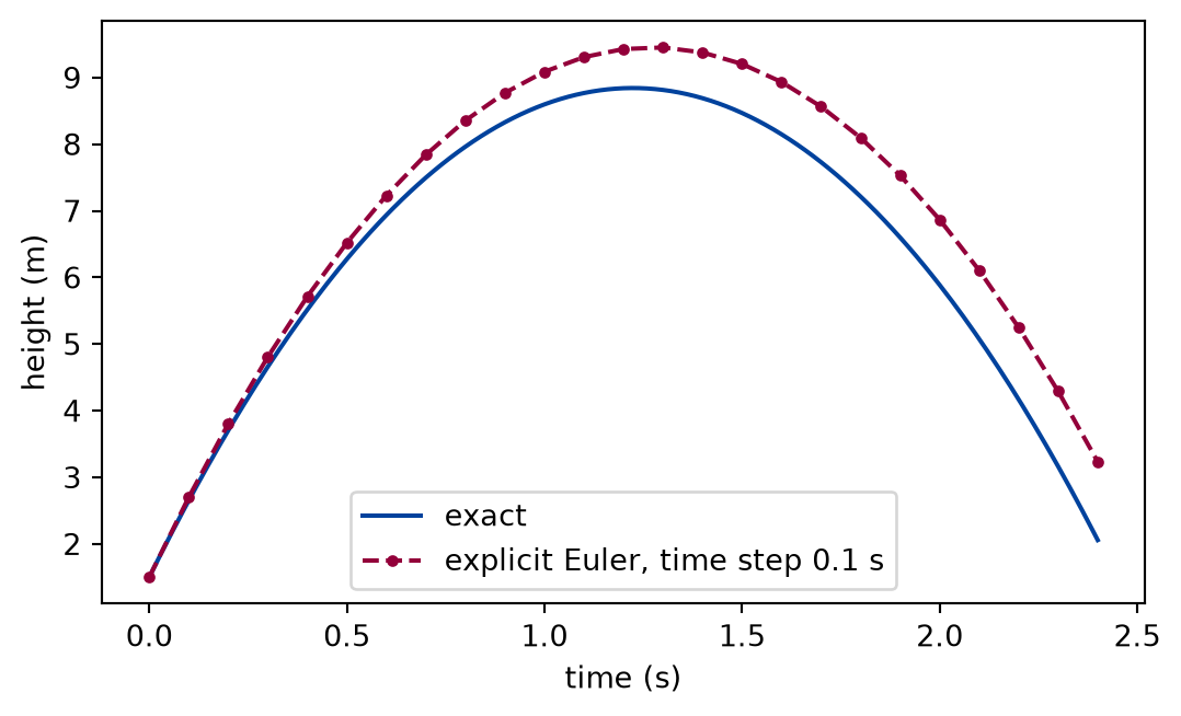
def draw_ball_thrown_up(euler: Trajectory) -> Figure:
    """The height of the ball: explicit Euler against the exact motion."""
    fine = np.linspace(0.0, euler.t[-1], 241)

    fig, ax = plt.subplots(figsize=(6.4, 3.6))
    ax.plot(
        fine,
        constant_acceleration(launch, -g, fine).x,
        color="#00429d",
        label="exact",
    )
    ax.plot(
        euler.t,
        euler.x,
        color="#93003a",
        linestyle="--",
        marker="o",
        markersize=3,
        label=f"explicit Euler, time step {dt} s",
    )
    ax.set_xlabel("time (s)")
    ax.set_ylabel("height (m)")
    ax.legend()
    return fig

src/pbc/mechanics/experiments/kinematics.py, lines 99 to 122, read from the repository when this page was built.

Figure 2: simulated Height of the ball: explicit Euler with a coarse time step against the exact motion. The simulated ball stays above the exact one by a gap that grows with time, the lag of a method that moves the ball with the velocity from the start of each step.

The Euler points start on the parabola and drift away from it, always on the same side, exactly as the formula predicts. Nothing in the figure suggests a different shape of motion: the whole difference is the lag of the position behind the velocity.

Halving the time step

A first-order method should halve its error when the time step halves. The cell repeats the simulation over the same duration, doubling the number of steps each time, and compares the final position with the exact one.

def final_error(acceleration, exact_position, n):
    """Error of the last simulated position, for n steps over the duration."""
    end = simulate(launch, acceleration, duration / n, n)
    return end.x[-1] - exact_position(end.t[-1])

src/pbc/mechanics/experiments/kinematics.py, lines 125 to 128, read from the repository when this page was built.

def halving(experiment: Experiment) -> np.ndarray:
    """The error of the final height for each time step; record its table."""
    ball_errors = np.array([final_error(free_fall, ball, n) for n in step_counts])

    experiment.table(
        "halving",
        [
            (
                n,
                duration / n,
                ball_errors[i],
                ball_errors[i - 1] / ball_errors[i] if i else None,
            )
            for i, n in enumerate(step_counts)
        ],
        columns=[
            ("steps", "", "d"),
            ("time step", "s", ".6f"),
            ("error", "m", ".6f"),
            ("previous error / error", "", ".4f"),
        ],
        caption="Error of the final height of the thrown ball for each time "
        "step, to six decimals, and the ratio to the error before the halving.",
    )
    return ball_errors

src/pbc/mechanics/experiments/kinematics.py, lines 131 to 155, read from the repository when this page was built.

Error of the final height of the thrown ball for each time step, to six decimals, and the ratio to the error before the halving.

steps	time step (s)	error (m)	previous error / error
24	0.100000	1.176798
48	0.050000	0.588399	2.0000
96	0.025000	0.294199	2.0000
192	0.012500	0.147100	2.0000
384	0.006250	0.073550	2.0000
768	0.003125	0.036775	2.0000

Every halving of the time step halves the error. For a constant acceleration the last ratio of the table is 2.0000, because the error is exactly $\tfrac{1}{2}\,g\,t\,\Delta t$.

The fifth assumption said that round-off stays far below the error of the method. The cell below puts a number on it: the spacing between neighbouring double-precision numbers at the height of the ball is 1.8e-15 m, and the smallest error of the table is 3.7e-02 m, which is 2.1e+13 times larger. Round-off begins to matter only for time steps far smaller than these.

An acceleration that changes in time

A constant acceleration is a special case: the computed velocity was exact. Take instead a cart on a shaking table, driven back and forth with $a(t) = a_0 \cos(\omega t)$ from rest. Integrating twice gives the exact motion

$$v(t) = \frac{a_0}{\omega} \sin(\omega t), \qquad x(t) = x_0 + \frac{a_0}{\omega^{2}} \bigl(1 - \cos(\omega t)\bigr).$$

The same simulate runs it; only the acceleration function changes.

a0 = 3.0  # amplitude of the acceleration, m/s^2
omega = 2.0  # angular frequency, rad/s
rest = State(t=0.0, x=0.0, v=0.0)

src/pbc/mechanics/experiments/kinematics.py, lines 34 to 36, read from the repository when this page was built.

def shaking_cart(experiment: Experiment) -> tuple[np.ndarray, np.ndarray]:
    """The error of the cart's final position for each time step, and the
    observed order; record their table."""
    cart_errors = np.array([cart_error(n) for n in step_counts])
    orders = np.log2(cart_errors[:-1] / cart_errors[1:])

    experiment.table(
        "shaking-cart",
        [
            (n, duration / n, cart_errors[i], orders[i - 1] if i else None)
            for i, n in enumerate(step_counts)
        ],
        columns=[
            ("steps", "", "d"),
            ("time step", "s", ".6f"),
            ("error", "m", ".6f"),
            ("observed order", "", ".3f"),
        ],
        caption="Error of the final position of the cart for each time step, "
        "to six decimals, and the observed order of the method to three decimals.",
    )
    return cart_errors, orders

src/pbc/mechanics/experiments/kinematics.py, lines 163 to 184, read from the repository when this page was built.

Error of the final position of the cart for each time step, to six decimals, and the observed order of the method to three decimals.

steps	time step (s)	error (m)	observed order
24	0.100000	0.497525
48	0.050000	0.251799	0.982
96	0.025000	0.126636	0.992
192	0.012500	0.063499	0.996
384	0.006250	0.031794	0.998
768	0.003125	0.015908	0.999

The observed order is the binary logarithm of the ratio of successive errors: one means the error halves with the time step. It is no longer exactly one, because the dropped terms now contain more than one power of $\Delta t$, but it approaches one as the step shrinks. With the smallest step the observed order is 0.999.

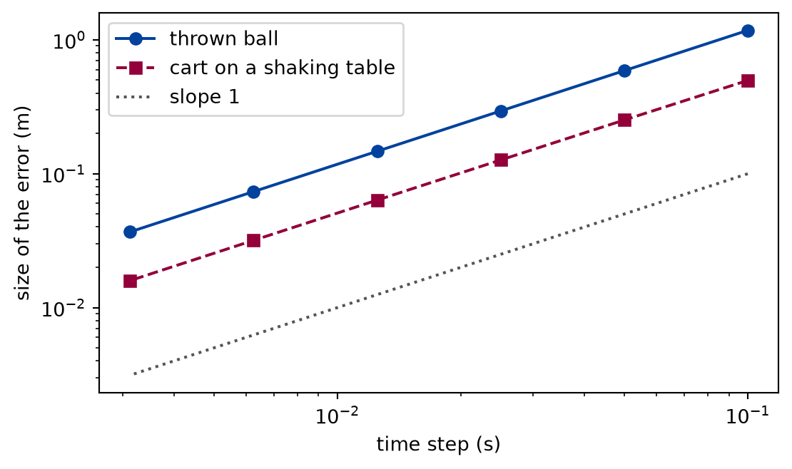
On logarithmic axes a first-order error is a straight line of slope one.

def draw_error_against_time_step(
    ball_errors: np.ndarray, cart_errors: np.ndarray
) -> Figure:
    """The error of the final position against the time step, log-log."""
    steps = duration / np.array(step_counts)

    fig, ax = plt.subplots(figsize=(6.4, 3.6))
    ax.loglog(
        steps, np.abs(ball_errors), color="#00429d", marker="o", label="thrown ball"
    )
    ax.loglog(
        steps,
        np.abs(cart_errors),
        color="#93003a",
        marker="s",
        linestyle="--",
        label="cart on a shaking table",
    )
    ax.loglog(steps, steps, color="#555555", linestyle=":", label="slope 1")
    ax.set_xlabel("time step (s)")
    ax.set_ylabel("size of the error (m)")
    ax.legend()
    return fig

src/pbc/mechanics/experiments/kinematics.py, lines 187 to 209, read from the repository when this page was built.

Figure 3: simulated Error of the final position against the time step, for both examples. Both fall along lines parallel to the reference line: the error is proportional to the time step.

Numerically verified (two motions): On logarithmic axes both errors follow the reference line of slope one, so the error of explicit Euler is proportional to the time step in both examples. The straight lines are the visible form of the first-order result; they say nothing about time steps far smaller or larger than the ones plotted.

Limits

What this lesson shows is a statement about one method on a few motions, not about numerical integration in general.

• The exact error formula holds for a constant acceleration only. For the cart the error is only approximately proportional to the time step, and the observed order approaches one as the step shrinks; it is not proved here for every smooth acceleration.
• The time steps stop where the errors are still far above round-off. The fifth assumption, that round-off is negligible, is stated, not tested: the lesson never shrinks the step far enough to see it matter.
• The acceleration is given as a function of time. Forces that depend on the position or velocity, such as a spring or drag, are not simulated, and the error behaves differently when the next step starts from a wrong state.
• An acceleration that jumps within a step, such as an impact, breaks the error estimate (fourth assumption), and nothing here measures by how much.
• Explicit Euler is the simplest method, not a good one. The exercises show a step that is exact for constant acceleration; the lesson on numerical integrators compares methods properly.

Self-check. Halving the time step halves the error of the thrown ball. Could you make the error as small as you like by halving again and again? Name what would change on the way.

1. Yes. Every halving halves the error, so the error can be made as small as you like.

   Not quite: this holds only in exact arithmetic. A computer rounds every step, and the rounding errors of many small steps add up.

2. No. At some time step the rounding errors become as large as the error of the method, and halving the step further no longer helps.

   Correct: this is the fifth assumption of the lesson. Round-off is negligible only for time steps that are not too small.

3. No. The error of the method does not depend on the time step at all.

   Not quite: the error of the method does shrink with the time step, in proportion to it. The limit comes from round-off, not from the method.

Solution to the self-check

In exact arithmetic yes: the error is proportional to the time step, so every halving halves it, at twice the work. A computer does not calculate exactly. Every step rounds its result, and with more and smaller steps these small rounding errors add up. At some time step the rounding error becomes as large as the error of the method, and halving the step further no longer helps. The first assumption of the lesson that fails is the fifth one: round-off is negligible only for time steps that are not too small.

Exercises

Exercise 1. Choose the time step. For the thrown ball of the first example, how small must the time step be for the position after 2.4 s to be within 1 mm of the exact one? Predict the answer from the error formula, then confirm it with a simulation.

Hint 1 of 2 for exercise 1

Solve the error formula for the time step, with the tolerance as the error.

Hint 2 of 2 for exercise 1

A simulation takes a whole number of steps. Which way must you round?

Solution to exercise 1

The error after the time $T$ is $\tfrac{1}{2}\,g\,T\,\Delta t$, so the time step must satisfy $\Delta t \le 2\,\varepsilon / (g\,T)$ for a tolerance $\varepsilon$. A simulation needs a whole number of steps, so we round the number of steps up.

def steps_for_tolerance(tolerance):
    """Exercise 1: the largest time step whose error stays within
    ``tolerance`` (m), the whole number of steps it takes, and their error."""
    largest_step = 2 * tolerance / (g * duration)
    n_needed = int(np.ceil(duration / largest_step))
    error_needed = final_error(free_fall, ball, n_needed)
    return largest_step, n_needed, error_needed

src/pbc/mechanics/experiments/kinematics.py, lines 212 to 218, read from the repository when this page was built.

largest time step: 85.0 microseconds
steps needed:      28244
error with them:   0.99997 mm

The simulation with 28244 steps ends 0.99997 mm from the exact position, just inside the tolerance. The first example used 24 steps. The error shrinks only in proportion to the work: that is the price of a first-order method.

Exercise 2. A constant jerk. A particle starts from rest at the origin and its acceleration grows linearly, $a(t) = j\,t$ with $j = 2$ m/s³. The exact motion is $v(t) = \tfrac{1}{2}\,j\,t^{2}$ and $x(t) = \tfrac{1}{6}\,j\,t^{3}$. Is the velocity computed by explicit Euler still exact? Measure the observed order of the position error at $t = 3$ s.

Hint 1 of 2 for exercise 2

Compare the acceleration at the start of a step with the acceleration during it. Does the velocity rule see the difference?

Hint 2 of 2 for exercise 2

The observed order is the base-two logarithm of the ratio of the errors of two runs, the second with half the time step of the first.

Solution to exercise 2

The velocity is no longer exact. Each step uses the acceleration at the start of the step, which is now smaller than the acceleration during the step, so the computed velocity falls behind.

jerk = 2.0  # m/s^3
end_time = 3.0  # s

src/pbc/mechanics/experiments/kinematics.py, lines 223 to 224, read from the repository when this page was built.

def jerk_errors(n):
    end = simulate(rest, growing, end_time / n, n)
    return (
        end.v[-1] - jerk * end.t[-1] ** 2 / 2,
        end.x[-1] - jerk * end.t[-1] ** 3 / 6,
    )

src/pbc/mechanics/experiments/kinematics.py, lines 232 to 237, read from the repository when this page was built.

def constant_jerk(experiment: Experiment) -> None:
    """Exercise 2: the velocity and position errors at ``end_time`` and the
    observed order; record their table."""
    counts = [30 * 2**k for k in range(5)]
    errors = np.array([jerk_errors(n) for n in counts])
    jerk_orders = np.log2(errors[:-1, 1] / errors[1:, 1])

    experiment.table(
        "constant-jerk",
        [
            (n, errors[i, 0], errors[i, 1], jerk_orders[i - 1] if i else None)
            for i, n in enumerate(counts)
        ],
        columns=[
            ("steps", "", "d"),
            ("velocity error", "m/s", ".6f"),
            ("position error", "m", ".6f"),
            ("observed order", "", ".3f"),
        ],
        caption="Velocity and position error of the cart with growing "
        "acceleration at t = 3 s, to six decimals, and the observed order.",
    )

src/pbc/mechanics/experiments/kinematics.py, lines 240 to 261, read from the repository when this page was built.

Velocity and position error of the cart with growing acceleration at t = 3 s, to six decimals, and the observed order.

steps	velocity error (m/s)	position error (m)	observed order
30	-0.300000	-0.880000
60	-0.150000	-0.445000	0.984
120	-0.075000	-0.223750	0.992
240	-0.037500	-0.112188	0.996
480	-0.018750	-0.056172	0.998

Both errors are negative: the computed particle is slower and has not come as far. Both halve with the time step, and the observed order of the position error tends to one.

Exercise 3. Keep one more term. The update rule dropped the term $\tfrac{1}{2}\,a(t)\,\Delta t^{2}$ from the position. Write a step that keeps it, and run the thrown ball of the first example again with its coarse time step of 0.1 s. What happens to the error, and why?

Hint 1 of 1 for exercise 3

The thrown ball has a constant acceleration. Which terms of the exact position does the new step now contain?

Solution to exercise 3

def second_order_step(state, acceleration, dt):
    """Exercise 3: an Euler step that keeps the term of the acceleration in
    the position."""
    a = acceleration(state.t)
    return State(
        t=state.t + dt,
        x=state.x + state.v * dt + 0.5 * a * dt**2,
        v=state.v + a * dt,
    )

src/pbc/mechanics/experiments/kinematics.py, lines 264 to 272, read from the repository when this page was built.

def improved_ball():
    """Exercise 3: the thrown ball with ``second_order_step``; the error of
    its final height."""
    state = launch
    for _ in range(n_steps):
        state = second_order_step(state, free_fall, dt)
    return state, state.x - ball(state.t)

src/pbc/mechanics/experiments/kinematics.py, lines 275 to 281, read from the repository when this page was built.

size of the error after 2.4 s: 0.000000000 m

The error drops from 1.177 m to zero in every digit shown; what is left is round-off. For a constant acceleration the Taylor expansion of the position ends after the $\Delta t^{2}$ term, so a step that keeps this term drops nothing. This holds for a constant acceleration only. For an acceleration that changes in time the expansion goes on, and the velocity is still updated by Euler’s rule, which is then no longer exact, as the previous exercise showed. An error remains.

Run this experiment

This page was built from commit 6417e2ff90258bd2d2ba21d217eb7666fd24f680 of the repository.

In a clone at that commit, with the project’s Python packages installed, this command runs the experiment of this page:

uv run --locked --no-dev python -m pbc.mechanics.experiments.kinematics results

Files, tests, and every command

The files behind it:

• site/lessons/mechanics/01-kinematics-as-a-program/index.qmd: this page, with every code cell.
• src/pbc/mechanics/kinematics.py: code the experiment runs.
• src/pbc/mechanics/experiments/kinematics.py: code the experiment runs.
• src/pbc/experiment.py: code the experiment runs.
• tests/unit/test_kinematics.py: tests of that code.
• tests/unit/test_kinematics_experiment.py: tests of that code.

With Git and uv installed (see the setup page), run:

git clone https://github.com/taspinar/physics-by-construction.git
cd physics-by-construction
git checkout 6417e2ff90258bd2d2ba21d217eb7666fd24f680
uv sync --locked --no-dev
uv run --locked --no-dev python -m pbc.mechanics.experiments.kinematics results

The experiment writes every figure of this page into results/, as <label>.png, and every number and table of the page, as the page shows it, into results/results.json. Its numbers match this page to the digits shown, and its figure files are the ones the page shows; digits beyond those can differ between machines, because floating-point libraries differ. Change the code of the experiment and run it again to see what changes.