Finite-volume methods and conservation laws

A conservation law computed as what flows through the faces of cells, with one interface for any system and a Riemann solver for each; the budgets of mass and momentum closed to round-off, the CFL limit, and a shock that the conservative scheme places right and a non-conservative one places wrong.

Course

Fluid dynamics, lesson 3 of 4

Slot

FL9, Finite-volume methods and conservation laws

Methods

Simulation

Difficulty

Intermediate, level 2 of 3

What you’ll learn

Write a conservation law in integral form and turn it into a finite-volume update of cell averages by face fluxes
Plug a Riemann solver for a system into one shared interface, and check the budgets of its conserved quantities to round-off
Choose the time step by the CFL condition and recognise what happens beyond it
Show that a non-conservative discretisation of the same equation converges to a wrong shock, and explain why

Prerequisites

Shock waves and the Burgers equation.

Before you begin

Calculus: the fundamental theorem, and integrals over an interval whose ends are fixed

Related

none

Previous

Shock waves and the Burgers equation

Next

Shallow-water equations: still water and the dam break

With scripts, this page keeps a record in your browser of whether you completed the lesson. Nothing is stored without them.

With scripts, this place suggests what to do next, with the reason, from the progress saved in your browser. Without them, follow the learning path.

A flood model that loses a few per cent of the water it was given, or a weather model that creates momentum out of nothing, gives wrong answers however fine its grid: the error does not go away, it accumulates. Mass, momentum, and energy are conserved in nature, and a program that moves them around should conserve them too, not approximately but by construction.

The finite-volume method does that. It does not approximate derivatives; it keeps the amount of each conserved quantity in each cell and moves amounts between neighbours, so what leaves one cell enters the next. This lesson builds the method once, as an interface into which any system plugs its own rule for the flux through a face, and uses it for the Burgers equation of the previous lesson and for the shallow-water equations of the next. It then checks three things: that the budgets close to the last digits, that the step must obey the CFL condition, and that a scheme which is not written as a difference of fluxes gets the speed of a shock wrong, on every grid.

Assumptions

One dimension, uniform cells. The cells are intervals of equal width. In two or three dimensions the faces are edges or areas and the method is the same; the geometry of the cells is not in this lesson.
First-order reconstruction. The state on each side of a face is the average of the cell on that side. A second-order method reconstructs a slope in each cell, with a limiter near shocks.
Explicit steps. Each step computes the fluxes from the state at the start of the step. The step is then limited by the CFL condition.
Conservation is of the model. The schemes conserve the quantities of the equations they discretise. Whether the equations describe the real flow is a separate question; a conservative scheme of the wrong model conserves the wrong things exactly.

From a conservation law to cells

The integral form

A conservation law for a vector of quantities $q(x, t)$ with the flux $f(q)$ is

$\frac{\partial q}{\partial t} + \frac{\partial f(q)}{\partial x} = 0 .$

Integrate it over a cell $[x_{j-1/2}, x_{j+1/2}]$ of width $\Delta x$ and over a step from $t_n$ to $t_{n+1}$ . With $Q_j$ the average of $q$ over the cell, the fundamental theorem of calculus gives, exactly,

$Q_j^{n+1} = Q_j^n - \frac{1}{\Delta x}\left(\int_{t_n}^{t_{n+1}} f\big(q(x_{j+1/2}, t)\big)\,\mathrm{d}t - \int_{t_n}^{t_{n+1}} f\big(q(x_{j-1/2}, t)\big)\,\mathrm{d}t\right).$

The integral form holds also where $q$ jumps, where the differential form has no meaning. A finite-volume method keeps this structure and approximates only the time integral of the flux through each face by $\Delta t\,F_{j+1/2}$ :

$Q_j^{n+1} = Q_j^n - \frac{\Delta t}{\Delta x}\left(F_{j+1/2} - F_{j-1/2}\right).$

Why the budget closes

Sum the update over all cells. Each interior face appears twice, once with a plus sign for the cell on its left and once with a minus for the cell on its right, and cancels. What is left is

$\Delta x \sum_j Q_j^{n+1} = \Delta x \sum_j Q_j^n + \Delta t\,\big(F_{\text{left end}} - F_{\text{right end}}\big).$

The total changes only by what flows through the two ends of the domain, whatever the fluxes are, as long as each face has one flux used by both of its cells. That is the budget the program checks. It is exact in arithmetic, so in floating point it closes to round-off, step after step. On a periodic domain the two ends are the same face and the total does not change at all.

The flux through a face: a Riemann problem

What flux crosses a face during a step? At the start of the step the state is constant in each cell, so at each face there is a jump from $Q_j$ to $Q_{j+1}$ . The solution of the conservation law from a single jump is the Riemann problem; the previous lesson solved it for Burgers’ equation: a shock or a fan. Godunov’s method takes the flux of that solution at the face. A system has one Riemann problem per pair of states, and each system has its own solver:

Burgers, exactly: the Godunov flux of the previous lesson.
Shallow water, approximately: the HLL flux keeps only the fastest wave to each side, with speeds $s_L$ and $s_R$ , and averages what lies between them so that the integral form holds: $F = \frac{s_R f(Q_L) - s_L f(Q_R) + s_L s_R\,(Q_R - Q_L)}{s_R - s_L} \quad\text{when } s_L < 0 < s_R .$
Any system, crudely: the Rusanov flux, $F = \tfrac12\big(f(Q_L) + f(Q_R)\big) - \tfrac12 a\,(Q_R - Q_L),$ with $a$ the largest signal speed of the two states. It needs only the flux and a bound on the speeds, and diffuses more than the others.

All three are functions of a left and a right state. That is the shared interface: the update, the boundaries, and the budget are written once, and a system supplies its Riemann solver.

The CFL condition

The Riemann solution at a face is valid as long as the waves from the two neighbouring faces do not reach it. The fastest wave moves at $\max|\lambda|$ , the largest signal speed (for Burgers $|u|$ , for shallow water $|u| + \sqrt{g h}$ ), so the step must satisfy

$\Delta t \le C_{\max}\,\frac{\Delta x}{\max|\lambda|},$

with the Courant number at most one. For Burgers’ equation with $C \le 1$ the Godunov scheme is total-variation diminishing: the sum of the jumps between neighbouring cells never grows, so no new oscillation appears. Beyond the limit the scheme uses a flux from a state the wave has already left, and nothing stops the solution from growing. The budget still closes, because it closes for any fluxes: conservation is not stability.

Conservative and non-conservative

Where $u$ is smooth, $\partial_x(u^2/2) = u\,\partial_x u$ , so the Burgers equation can also be discretised as an upwind difference of $u$ times $u$ :

$u_j^{n+1} = u_j^n - \frac{\Delta t}{\Delta x}\,u_j^n\,(u_j^n - u_{j-1}^n) \qquad (u > 0).$

It is consistent: for smooth $u$ it differs from the equation by terms that vanish with $\Delta x$ . But it is not a difference of fluxes, so the sum over the cells does not telescope, and nothing makes it conserve $u$ across a jump, where $u$ is not smooth. The Lax-Wendroff theorem says that a conservative and consistent scheme that converges converges to a weak solution, one that satisfies the integral form and hence the Rankine-Hugoniot speed. A non-conservative scheme has no such guarantee, and the third example shows it converging to a shock at another speed.

Code

interface_fluxes adds the ghost cells of the boundary and calls the Riemann solver on every face at once; conservative_update is the update by flux differences; evolve chooses each step by the CFL condition and records the totals and what entered through the ends.

def interface_fluxes(q: Array, riemann: RiemannSolver, boundary: Boundary) -> Array:
    """The flux through each of the n + 1 faces of the n cells, the first face
    at the left end of the domain and the last at the right end."""
    padded = with_ghosts(q, boundary)
    return riemann(padded[:-1], padded[1:])

src/pbc/fluids/finite_volume.py, lines 62 to 66, read from the repository when this page was built.

def conservative_update(q: Array, fluxes: Array, dt: float, dx: float) -> Array:
    """One step of the cell averages from the fluxes through their faces:
    each cell gains what enters through its left face and loses what leaves
    through its right face."""
    return q - dt / dx * (fluxes[1:] - fluxes[:-1])

src/pbc/fluids/finite_volume.py, lines 69 to 73, read from the repository when this page was built.

def evolve(
    q0: Array,
    dx: float,
    t_end: float,
    fluxes: Callable[[Array], Array],
    max_speed: Callable[[Array], float],
    courant: float,
    source: Callable[[Array], Array] | None = None,
) -> Run:
    """Advance the cell averages ``q0`` from the time 0 to ``t_end`` with
    steps chosen by the CFL condition: dt = ``courant`` dx / ``max_speed``,
    the last step shortened to end at ``t_end``. ``fluxes(q)`` returns the
    n + 1 face fluxes of the state (``interface_fluxes`` with a Riemann
    solver and a boundary); ``source(q)``, if given, is added as dt times
    its value, computed from the same state as the fluxes. A state with no
    wave speed (all zero, or fully dry) bounds no step: it is left as it is
    and the run jumps to ``t_end`` in one step with no flux and no source."""
    q = np.array(q0, dtype=float)
    t = 0.0
    times = [t]
    totals = [q.sum(axis=0) * dx]
    inflow = [np.zeros_like(totals[0])]
    while t < t_end:
        speed = max_speed(q)
        if speed == 0.0:
            times.append(t_end)
            totals.append(totals[-1])
            inflow.append(inflow[-1])
            break
        dt = min(courant * dx / speed, t_end - t)
        face = fluxes(q)
        added = None if source is None else source(q)
        q = conservative_update(q, face, dt, dx)
        if added is not None:
            q = q + dt * added
        t = t_end if t + dt >= t_end else t + dt
        times.append(t)
        totals.append(q.sum(axis=0) * dx)
        inflow.append(inflow[-1] + dt * (face[0] - face[-1]))
    return Run(q=q, t=np.array(times), totals=np.array(totals), inflow=np.array(inflow))

src/pbc/fluids/finite_volume.py, lines 116 to 155, read from the repository when this page was built.

The shallow-water system plugs in through hll_flux, with the wave speeds of Einfeldt; its equations are derived in the next lesson.

def hll_flux(left: Array, right: Array) -> Array:
    """The HLL flux through a face: the exact flux of a Riemann solution
    reduced to its two outermost waves, with the speeds of Einfeldt (the
    extreme of the characteristic speeds of the two states and of their Roe
    average). Where both waves move the same way the face sees the upstream
    flux."""
    h_left, h_right = left[:, 0], right[:, 0]
    u_left, u_right = velocity(left), velocity(right)
    c_left, c_right = np.sqrt(GRAVITY * h_left), np.sqrt(GRAVITY * h_right)
    root_left, root_right = np.sqrt(h_left), np.sqrt(h_right)
    roots = root_left + root_right
    wet = roots > 0
    safe = np.where(wet, roots, 1.0)
    u_roe = np.where(wet, (root_left * u_left + root_right * u_right) / safe, 0.0)
    c_roe = np.sqrt(0.5 * GRAVITY * (h_left + h_right))
    slow = np.minimum(np.minimum(u_left - c_left, u_right - c_right), u_roe - c_roe)
    fast = np.maximum(np.maximum(u_left + c_left, u_right + c_right), u_roe + c_roe)
    f_left, f_right = flux(left), flux(right)
    span = np.where(fast > slow, fast - slow, 1.0)
    middle = (
        fast[:, None] * f_left
        - slow[:, None] * f_right
        + (slow * fast)[:, None] * (right - left)
    ) / span[:, None]
    return np.where(
        slow[:, None] >= 0, f_left, np.where(fast[:, None] <= 0, f_right, middle)
    )

src/pbc/fluids/shallow_water.py, lines 68 to 94, read from the repository when this page was built.

Worked examples

Budgets to round-off

Four runs on two hundred cells: Burgers’ equation with a smooth wave on a periodic domain until well after it breaks, and with a jump between open ends; the shallow-water equations with a hump of water moving on a periodic domain, and with a dam break in a tank with walls at both ends. Each records the total of each conserved quantity and what entered through the ends, at every step.

LENGTH = 1.0  # m
BUDGET_CELLS = 200
BUDGET_BOUND = 1e-13  # relative to the size of the totals at the start

src/pbc/fluids/experiments/finite_volume_methods_and_conservation_laws.py, lines 31 to 33, read from the repository when this page was built.

def budget_run(experiment: Experiment) -> float:
    """The change of each total and the largest residual of its budget, for
    each case; record the table and return the largest relative residual."""
    rows = []
    worst = 0.0
    for system, boundary, names, run in budget_cases():
        totals = run.totals.reshape(len(run.t), -1)
        scale = np.abs(totals[0]) + 1.0
        residual = np.max(np.abs(run.budget_residual.reshape(len(run.t), -1)), axis=0)
        for i, name in enumerate(names):
            relative = float(residual[i] / scale[i])
            worst = max(worst, relative)
            # Rounded to the table's four decimals with the sign of zero removed,
            # so that a change of -1e-17 shows as "0.0000", never "-0.0000".
            change = round(float(totals[-1, i] - totals[0, i]), 4) + 0.0
            rows.append((system, boundary, name, change, f"below {BUDGET_BOUND:.0e}"))
    assert worst < BUDGET_BOUND, "a budget did not close"
    experiment.table(
        "budget-run",
        rows,
        [
            ("system", "", ""),
            ("ends", "", ""),
            ("quantity", "", ""),
            ("change of the total", "", ".4f"),
            ("largest budget residual", "", ""),
        ],
        "For each run: the change of the total of each conserved quantity over "
        "the run, in the units of the quantity times metres, and the largest "
        "difference, over all steps, between that change and what entered "
        "through the ends, relative to the total at the start plus one.",
    )
    return worst

src/pbc/fluids/experiments/finite_volume_methods_and_conservation_laws.py, lines 89 to 121, read from the repository when this page was built.

For each run: the change of the total of each conserved quantity over the run, in the units of the quantity times metres, and the largest difference, over all steps, between that change and what entered through the ends, relative to the total at the start plus one.
system	ends	quantity	change of the total	largest budget residual
Burgers	periodic	u	0.0000	below 1e-13
Burgers	open	u	0.5625	below 1e-13
shallow water	periodic	h	0.0000	below 1e-13
shallow water	periodic	hu	0.0000	below 1e-13
shallow water	walls	h	0.0000	below 1e-13
shallow water	walls	hu	-0.2170	below 1e-13

Numerically verified (Burgers with the Godunov flux and shallow water with the HLL flux, the four runs of the table): With the face fluxes of the shared interface, the change of the total of every conserved quantity equals what entered through the ends, to round-off, at every step, for both systems and every kind of end. The open Burgers run gains $u$ because more enters on the fast side than leaves on the slow side; the periodic runs keep their totals. In the tank the water’s mass stays fixed while its momentum changes: the walls push on the water, and that push is the momentum flux through the end faces, mostly the pressure $g h^2/2$ of the water against the wall, which the budget counts. A budget does not say that the momentum is conserved; it says that it changes only by what the ends let through.

The CFL limit

The smooth wave of the first run, now with the step chosen at six Courant numbers from one half to two.

courants = [0.5, 0.9, 1.0, 1.3, 1.6, 2.0]
COURANT_TIME = 1.0  # s

src/pbc/fluids/experiments/finite_volume_methods_and_conservation_laws.py, lines 37 to 38, read from the repository when this page was built.

The smooth wave of the budget example, run for one second with the Godunov flux at each Courant number: its total variation and its largest value at the end, each over its value at the start.
Courant number	total variation, end over start	largest value, end over start
0.5	0.693	0.897
0.9	0.710	0.904
1.0	0.715	0.907
1.3	1.097	0.934
1.6	3.284	2.326
2.0	188.414	125.599

Numerically verified (the smooth wave of the first example, one second, the Courant numbers of the table): Within the CFL condition, $C \le 1$ , the Godunov scheme for Burgers’ equation does not increase the total variation or the largest value of the solution; beyond it both can grow without bound, while the budget still closes to round-off. Up to $C = 1$ the total variation falls, as the shock that forms absorbs the wave, and no value exceeds the largest at the start. Just beyond, the guarantee is gone and the variation rises; at the largest steps the solution blows up. Every one of these runs, the unstable ones included, closes its budget below 1e-13: a conservative scheme can be perfectly conservative and worthless.

Conservative and non-conservative schemes

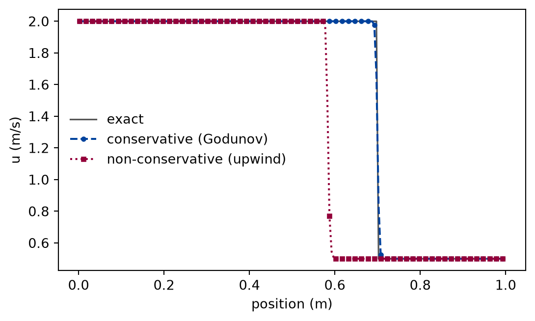
A jump from two to one half metres per second, which the Rankine-Hugoniot condition makes a shock of speed 1.2500 m/s, run for four tenths of a second by the conservative Godunov scheme and by the non-conservative upwind scheme, on grids from one hundred to sixteen hundred cells.

LEFT, RIGHT = 2.0, 0.5  # m/s
START = 0.2  # m
END_TIME = 0.4  # s
cells = [100, 200, 400, 800, 1600]
COURANT = 0.9

src/pbc/fluids/experiments/finite_volume_methods_and_conservation_laws.py, lines 42 to 46, read from the repository when this page was built.

def nonconservative_step(u: Array, dt: float, dx: float, boundary: Boundary) -> Array:
    """One upwind step of the form u_t + u u_x = 0: the difference of u is
    taken on the side the wave comes from, and multiplied by the local u.
    It is the same equation where u is smooth, but it is not a difference of
    fluxes, so nothing makes what leaves one cell enter the next."""
    padded = with_ghosts(u, boundary)
    backward = padded[1:-1] - padded[:-2]
    forward = padded[2:] - padded[1:-1]
    return u - dt / dx * u * np.where(u > 0, backward, forward)

src/pbc/fluids/burgers.py, lines 113 to 121, read from the repository when this page was built.

def nonconservative(n: int) -> tuple[np.ndarray, float]:
    """The jump run with the non-conservative upwind step on ``n`` cells: the
    profile at the end, and the mass it created per unit time, the change of
    the total minus what the fluxes at the two ends brought in."""
    dx = LENGTH / n
    u = np.where(centres(n) < START, LEFT, RIGHT)
    mass = float(np.sum(u) * dx)
    entered = 0.0
    t = 0.0
    while t < END_TIME:
        dt = min(COURANT * dx / burgers.max_speed(u), END_TIME - t)
        entered += dt * float(burgers.flux(u[0]) - burgers.flux(u[-1]))
        u = burgers.nonconservative_step(u, dt, dx, transmissive)
        t = END_TIME if t + dt >= END_TIME else t + dt
    return u, (float(np.sum(u) * dx) - mass - entered) / END_TIME

src/pbc/fluids/experiments/finite_volume_methods_and_conservation_laws.py, lines 175 to 189, read from the repository when this page was built.

The jump from two to one half metres per second after four tenths of a second, computed by the conservative Godunov scheme and by the non-conservative upwind scheme on each grid: the integral of the absolute error over the domain, and the speed of the shock from its position.
cells	error, conservative (m²/s)	error, non-conservative (m²/s)	shock speed, conservative (m/s)	shock speed, non-conservative (m/s)
100	7.12e-03	1.77e-01	1.2499	0.9536
200	3.69e-03	1.73e-01	1.2500	0.9606
400	1.91e-03	1.72e-01	1.2500	0.9632
800	8.91e-04	1.71e-01	1.2500	0.9648
1600	4.62e-04	1.71e-01	1.2500	0.9655

Numerically verified (the jump of the example, Burgers' equation, Courant number nine tenths): The conservative scheme converges to the exact shock with order one; the non-conservative scheme converges to a shock at another speed, and its error does not fall as the grid is refined. The fitted orders are 0.99 and 0.01. The non-conservative shock settles at 0.966 m/s, and refining the grid only sharpens it there. The scheme creates $u$ at the rate -0.427 $\mathrm{m^2/s^2}$ , measured from its budget, which is exactly the speed difference times the jump, -0.427 $\mathrm{m^2/s^2}$ : the shock is slow because the scheme loses the quantity whose conservation fixes the speed.

def draw_conservative_and_not() -> Figure:
    """The jump after the run on two hundred cells: the exact solution, the
    conservative scheme, and the non-conservative scheme."""
    n = 200
    x = centres(n)
    exact = burgers.riemann_solution(LEFT, RIGHT, (x - START) / END_TIME)
    good = conservative(n)
    bad, _ = nonconservative(n)
    fig, ax = plt.subplots(figsize=(6.4, 3.6))
    ax.plot(x, exact, color=FIGURE_COLOURS[2], linewidth=1.2, label="exact")
    ax.plot(
        x,
        good,
        color=FIGURE_COLOURS[0],
        linestyle="--",
        marker="o",
        markersize=3,
        markevery=3,
        label="conservative (Godunov)",
    )
    ax.plot(
        x,
        bad,
        color=FIGURE_COLOURS[1],
        linestyle=":",
        marker="s",
        markersize=3,
        markevery=3,
        label="non-conservative (upwind)",
    )
    ax.set_xlabel("position (m)")
    ax.set_ylabel("u (m/s)")
    ax.legend(loc="center left", frameon=False)
    return fig

src/pbc/fluids/experiments/finite_volume_methods_and_conservation_laws.py, lines 253 to 286, read from the repository when this page was built.

Line plot of the velocity u against position. The exact solution is a step down from the higher to the lower state. The conservative points follow it, with the step at the same place. The non-conservative points also form a sharp step, but well to the left of the exact one. — Figure 1: simulated The same jump after the same time, computed from the same equation in two forms: the conservative scheme puts the shock where the exact solution has it, the non-conservative scheme leaves it behind.

Both computed shocks are sharp, and nothing in the picture of the non-conservative one looks wrong: it is a clean jump between the right states, in the wrong place. The data are simulated on two hundred cells, and the reference is the exact solution of the Riemann problem.

Limits

Conservation is not accuracy. A budget that closes says the scheme moves the quantities without losing any. It says nothing about where it moves them: the unstable runs of the second example close their budgets, and so would a scheme with far too much numerical diffusion.
Conservation is of the discretised model. The shallow-water equations conserve the momentum of a depth-averaged flow over a flat bed; a real river has friction and a bed that pushes back, and its budget has terms that the model of this lesson does not.
First order. The errors fall with the first power of the cell width. Reconstructing slopes gives second order away from shocks; at a shock every method is first order in this error measure.
The CFL condition is necessary, not sufficient. It keeps the waves of one face from reaching the next. Stability of a particular scheme, and positivity of a depth, need more, as the next lesson shows for the depth.

Self-check. A scheme for a conservation law closes its budget to round-off at every step. What can you conclude?

The scheme is stable, because a solution that grows would change the total.

A solution can grow in some cells and fall in others with the same total; the unstable runs of the CFL example closed their budgets.
The scheme is written as a difference of face fluxes, so any shocks it converges to move at the Rankine-Hugoniot speed; stability and accuracy are separate questions.

Correct: conservation fixes the shock speed of a converging scheme (the Lax-Wendroff theorem), and nothing else.
The computed solution is the physical one.

The scheme conserves the quantities of its model. A wrong model, an unstable step, or too coarse a grid all close their budgets.

Solution to the self-check

Only that the scheme is conservative: one flux per face, shared by its two cells. That is what makes a convergent scheme converge to a solution with the right shock speeds. It guarantees neither stability (the CFL example) nor accuracy, nor that the model describes the real flow.

Exercises

Exercise 1. Two Riemann solvers. Compute the jump of the third example on $400$ cells with the Godunov and the Rusanov flux, and also the smooth wave of the first example at $0.2$ s, before it breaks. Do the two fluxes put the shock in the same place? Which is more accurate?

Hint 1 of 1 for exercise 1

The Rusanov flux plugs into the same interface; it needs only the flux and a bound on the signal speed.

Solution to exercise 1

def rusanov_run(experiment: Experiment) -> None:
    """Exercise 1: the jump on four hundred cells and the smooth wave of the
    budget example before it breaks, with the Godunov and the Rusanov flux;
    record the speed of the shock and the error of each run."""
    n = 400
    dx = LENGTH / n
    x = centres(n)
    exact = burgers.riemann_solution(LEFT, RIGHT, (x - START) / END_TIME)
    wave = 1.0 + 0.5 * np.sin(2.0 * np.pi * x)
    smooth = burgers.characteristic_solution(
        lambda y: 1.0 + 0.5 * np.sin(2.0 * np.pi * y), x, 0.2, LENGTH
    )
    rows = []
    for name, riemann in (
        ("Godunov", burgers.godunov_flux),
        ("Rusanov", rusanov(burgers.flux, np.abs)),
    ):
        u = conservative(n, riemann)
        v = evolve(
            wave,
            dx,
            0.2,
            lambda w, riemann=riemann: interface_fluxes(w, riemann, periodic),
            burgers.max_speed,
            COURANT,
        ).q
        rows.append(
            (name, (shock_position(u, x) - START) / END_TIME,
             float(np.sum(np.abs(u - exact)) * dx),
             float(np.sum(np.abs(v - smooth)) * dx))
        )  # fmt: skip
    experiment.table(
        "rusanov-run",
        rows,
        [
            ("flux", "", ""),
            ("shock speed", "m/s", ".4f"),
            ("error at the shock", "m²/s", ".2e"),
            ("error of the smooth wave", "m²/s", ".2e"),
        ],
        "Two Riemann solvers on four hundred cells: the speed of the shock of "
        "the comparison and the integral of its absolute error, and the "
        "integral of the absolute error of the smooth wave of the budget "
        "example before it breaks.",
    )

src/pbc/fluids/experiments/finite_volume_methods_and_conservation_laws.py, lines 289 to 333, read from the repository when this page was built.

Two Riemann solvers on four hundred cells: the speed of the shock of the comparison and the integral of its absolute error, and the integral of the absolute error of the smooth wave of the budget example before it breaks.
flux	shock speed (m/s)	error at the shock (m²/s)	error of the smooth wave (m²/s)
Godunov	1.2500	1.91e-03	1.49e-03
Rusanov	1.2503	2.72e-03	1.51e-03

Both shocks move at the Rankine-Hugoniot speed: both schemes are conservative, so the speed is not theirs to choose. The Rusanov flux adds more diffusion at the shock, where the two states differ much, and has the larger error there. In the smooth wave the neighbouring states nearly agree and the two fluxes nearly coincide.

Exercise 2. The same scheme, written conservatively. For a jump in which $u$ is positive everywhere, the upwind scheme can be written as a difference of fluxes, $u_j^{n+1} = u_j^n - \frac{\Delta t}{\Delta x}\left(u_j^2/2 - u_{j-1}^2/2\right)$ . Put it into the shared interface and measure the shock speed of the third example on the finest grid.

Hint 1 of 1 for exercise 2

The face flux is the flux of the state on its left, whatever the state on its right.

Solution to exercise 2

def upwind_flux_speed() -> float:
    """Exercise 2: the shock speed of the upwind scheme written as a
    difference of fluxes, on the finest grid; every state of the jump is
    positive, so the upwind face takes the flux of its left cell."""
    n = cells[-1]
    u = conservative(n, lambda left, right: burgers.flux(left))
    return (shock_position(u, centres(n)) - START) / END_TIME

src/pbc/fluids/experiments/finite_volume_methods_and_conservation_laws.py, lines 336 to 342, read from the repository when this page was built.

The shock moves at 1.2500 m/s, the Rankine-Hugoniot speed, where the non-conservative form of the same upwind difference gave 0.966 m/s. The two schemes agree to first order wherever $u$ is smooth; they differ only in whether the change of a cell is a difference of fluxes, and at a shock that is all that matters.

Run this experiment

This page was built from commit 3a83ab640162bf2b624c2b254d917ed5bdc7090d of the repository.

In a clone at that commit, with the project’s Python packages installed, this command runs the experiment of this page:

uv run --locked --no-dev python -m pbc.fluids.experiments.finite_volume_methods_and_conservation_laws results

Files, tests, and every command

The files behind it:

site/lessons/fluids/03-finite-volume-methods-and-conservation-laws/index.qmd: this page, with every code cell.
src/pbc/fluids/finite_volume.py: code the experiment runs.
src/pbc/fluids/burgers.py: code the experiment runs.
src/pbc/fluids/shallow_water.py: code the experiment runs.
src/pbc/fluids/experiments/finite_volume_methods_and_conservation_laws.py: code the experiment runs.
src/pbc/verification/estimates.py: code the experiment runs.
src/pbc/experiment.py: code the experiment runs.
tests/unit/test_fluids.py: tests of that code.
tests/unit/test_finite_volume_methods_and_conservation_laws_experiment.py: tests of that code.

With Git and uv installed (see the setup page), run:

git clone https://github.com/taspinar/physics-by-construction.git
cd physics-by-construction
git checkout 3a83ab640162bf2b624c2b254d917ed5bdc7090d
uv sync --locked --no-dev
uv run --locked --no-dev python -m pbc.fluids.experiments.finite_volume_methods_and_conservation_laws results

The experiment writes every figure of this page into results/, as <label>.png, and every number and table of the page, as the page shows it, into results/results.json. Its numbers match this page to the digits shown, and its figure files are the ones the page shows; digits beyond those can differ between machines, because floating-point libraries differ. Change the code of the experiment and run it again to see what changes.