The chirp law, proved

The shrinking orbit, the rate of the frequency, the chirp mass, and the time to coalescence of the gravitational-wave strain lab, stated and proved in Lean 4 as exact consequences of Kepler’s third law and an assumed energy loss, and what that says about the model and nothing about the measurement.

Course

Classical mechanics, lesson 28 of 28

Methods

Formal proofs

Difficulty

Advanced, level 3 of 3

What you’ll learn

State the shrink rate of a circular orbit and the chirp rate as theorems in Lean 4, with the quadrupole power as a hypothesis
Read the proof that a frequency and its rate fix the chirp mass, and the proof that the time to coalescence counts down at the rate one
Say that the theorems are about the model of the lab, and that they prove nothing about the measured strain or the masses of the black holes

Prerequisites

Gravitational-wave strain lab, Proving what the simulation showed.

Before you begin

Calculus: the chain rule and the derivative of a power and of a quotient

Related

none

Previous

Lean exercises on your machine

Next

none yet; this is the last lesson of the learning path so far

With scripts, this page keeps a record in your browser of whether you completed the lesson. Nothing is stored without them.

With scripts, this place suggests what to do next, with the reason, from the progress saved in your browser. Without them, follow the learning path.

The gravitational-wave strain lab derives the chirp of two bodies that spiral together, from Kepler’s third law and one input from outside Newtonian mechanics, the power that the pair radiates. It then checks the result against a numerical inspiral for one pair of masses. A check for one pair of masses does not show that the algebra holds for every pair, and a slip in a long chain of fractional powers is easy to make. This lesson states the steps in Lean and proves them for all masses at once.

It proves properties of the model: the equations of the lab and what follows from them. It does not prove anything about the strain that the detectors recorded, about the fit, or about the black holes. That limit comes back at the end, and it is the main one.

Assumptions

Every assumption is a hypothesis of a theorem or a definition; the build fails on sorry and on any axiom the project declares.

Two point masses on a circular orbit. The separation $a$ is the only coordinate. Kepler’s third law holds at every instant, $\omega^2 a^3 = G(m_1 + m_2)$ with $\omega = \pi f$ the orbital angular frequency (hK). The orbit is assumed to stay circular while it shrinks.
The quadrupole power is an assumption, not derived. The energy of the orbit is $-G m_1 m_2/(2a)$ (orbitEnergy), and it falls at the power $\tfrac{32}{5} G^4 m_1^2 m_2^2 (m_1+m_2)/(c^5 a^5)$ (quadrupolePower), the formula of general relativity. The hypothesis hloss says that the derivative of the energy is minus that power. Nothing in the proofs justifies the power; a different power gives a different shrink rate.
Positive constants and masses. hG, hc, hm₁, hm₂, and a positive separation ha0. They let the proofs divide.
The chirp mass by its fifth power. hMc5 defines $\mathcal{M}$ through $\mathcal{M}^5 = (m_1 m_2)^3/(m_1+m_2)$ . Powers in the theorems are whole numbers: the lab’s $\omega^{11/3}$ appears as the cube of the rate, $(\omega')^3 \propto \omega^{11}$ , which says the same thing without a fractional power of a real number.
Differentiable in time. The separation and the frequency have derivatives at the instant considered (HasDerivAt). The theorems are about those derivatives and not about a numerical integration.
Real numbers, not floating-point numbers. Lean’s ℝ has no round-off, and the constants $G$ and $c$ are arbitrary positive reals, not the measured values.

What the theorems say

Write $\mathcal{M}$ for the chirp mass and $\omega = \pi f$ . The lab’s chain of steps is proved in pieces.

The orbit shrinks. If the separation has the derivative $a'$ and the energy $-G m_1 m_2/(2a)$ has the derivative $-P(a)$ , the chain rule gives $\tfrac{G m_1 m_2}{2 a^2}\,a' = -P(a)$ , and so

$a' = -\frac{64}{5}\,\frac{G^3 m_1 m_2 (m_1 + m_2)}{c^5 a^3}.$

The frequency rises. Differentiating Kepler’s law, $\omega^2 a^3 = G(m_1+m_2)$ , along the orbit gives $2\omega\omega' a^3 + 3\omega^2 a^2 a' = 0$ , so $\omega' = -\tfrac{3\omega}{2a}\,a'$ . With the shrink rate, and Kepler’s law again to remove $a$ , the masses enter only through $\mathcal{M}$ :

$(\omega')^3 = \left(\frac{96}{5}\right)^3 \left(\frac{G\mathcal{M}}{c^3}\right)^5 \omega^{11}.$

The chirp mass can be read back. The same relation gives $(G\mathcal{M}/c^3)^5 = (5/96)^3(\omega')^3/\omega^{11}$ , and a positive $\mathcal{M}$ is fixed by its fifth power: a frequency and its rate cannot belong to two different chirp masses.

The time to coalescence. If $(\omega')^3 = K\omega^{11}$ holds on a neighbourhood of an instant $t$ , then $\tau = 3\omega/(8\omega')$ has the derivative $-1$ at $t$ : it is a clock that counts down at the rate one. This is a local identity. If the inspiral runs on until the frequency diverges, $\tau$ reaches zero there, which is the coalescence time of the lab, $(5/256)(\pi f)^{-8/3}(G\mathcal{M}/c^3)^{-5/3}$ ; that the inspiral reaches the divergence is not proved here.

Formal theorem (two positive masses on a circular orbit, the quadrupole power taken as a hypothesis, real arithmetic): If a circular orbit loses energy at the quadrupole power, its separation shrinks at the rate $-\tfrac{64}{5}G^3 m_1 m_2 (m_1+m_2)/(c^5 a^3)$ .

Formal theorem (the same model, real arithmetic): With Kepler’s third law, the rate of change of the orbital angular frequency satisfies $(\omega')^3 = (96/5)^3 (G\mathcal{M}/c^3)^5\omega^{11}$ with the chirp mass defined by $\mathcal{M}^5 = (m_1 m_2)^3/(m_1 + m_2)$ .

Formal theorem (positive constants, a non-zero frequency, real arithmetic): A frequency and its rate of change determine the chirp mass: two positive chirp masses that satisfy the law with the same $\omega$ and $\omega'$ are equal.

Formal theorem (a local identity at one instant, for a rising frequency with a differentiable rate, real arithmetic): Where $(\omega')^3 = K\omega^{11}$ holds on a neighbourhood of an instant, the quantity $3\omega/(8\omega')$ decreases at the rate one at that instant.

The proofs

The listings are read from the Lean files of the repository when the site is built, and they are the text that lake build compiled.

Compiled with Lean 4.34.1 and Mathlib v4.34.1: ./scripts/check-lean.sh found no sorry and no axiom declared by the project before this page was built.

Commit 6417e2ff90258bd2d2ba21d217eb7666fd24f680 of the repository.

What was checked, and where to read the proofs

./scripts/check-lean.sh ran lake build on every module of the project and found no sorry and no axiom declared by the project before this page was built. CI runs the same check on every pull request and on main.

Lean 4.34.1, from the toolchain pinned in lean/lean-toolchain.
Mathlib v4.34.1, revision d13f23b723.
lean/PhysicsByConstruction/Mechanics/Chirp.lean, or open it in the Lean web editor

The file in the repository at that commit and the result of the CI run are authoritative. The Lean web editor is a convenience: it runs its own version of Mathlib, which can differ from the one above, so a proof that compiled here may report an error there.

The definitions. The power is a definition, and its use is a hypothesis of the next theorem.

/-- The energy of a circular orbit of separation `a`: `-G m₁ m₂ / (2 a)`. -/
noncomputable def orbitEnergy (G m₁ m₂ a : ℝ) : ℝ :=
  -(G * m₁ * m₂) / (2 * a)

/-- The power of the quadrupole formula radiated by a circular orbit of
separation `a`, `(32/5) G⁴ m₁² m₂² (m₁ + m₂) / (c⁵ a⁵)`. An assumption of the
model, taken from general relativity. -/
noncomputable def quadrupolePower (G c m₁ m₂ a : ℝ) : ℝ :=
  32 / 5 * G ^ 4 * m₁ ^ 2 * m₂ ^ 2 * (m₁ + m₂) / (c ^ 5 * a ^ 5)

lean/PhysicsByConstruction/Mechanics/Chirp.lean, lines 40 to 48, read from the repository when this page was built.

The shrink rate. hloss is the assumption: the energy of the orbit falls at the quadrupole power. The proof compares two derivatives of the same function, the one the chain rule gives and the one hloss states, and clears the denominators.

/-- **The orbit shrinks at the rate the energy loss fixes.** If the separation
`a` of a circular orbit has the derivative `a'` at `t`, and the energy of the
orbit has the derivative `-P` there (`hloss`, the loss at the quadrupole
power), then `a' = -(64/5) G³ m₁ m₂ (m₁ + m₂) / (c⁵ a³)`. -/
theorem shrink_rate_of_energy_loss
    (G c m₁ m₂ : ℝ) (a : ℝ → ℝ) (a' t : ℝ)
    (hG : 0 < G) (hc : 0 < c) (hm₁ : 0 < m₁) (hm₂ : 0 < m₂) (ha0 : 0 < a t)
    (ha : HasDerivAt a a' t)
    (hloss : HasDerivAt (fun s => orbitEnergy G m₁ m₂ (a s))
      (-quadrupolePower G c m₁ m₂ (a t)) t) :
    a' = -(64 / 5) * G ^ 3 * m₁ * m₂ * (m₁ + m₂) / (c ^ 5 * a t ^ 3) := by
  have hne : a t ≠ 0 := ha0.ne'
  have h1 : HasDerivAt (fun s => 2 * a s) (2 * a') t := ha.const_mul 2
  have h2 : HasDerivAt (fun s => (2 * a s)⁻¹) (-(2 * a') / (2 * a t) ^ 2) t :=
    h1.inv (by positivity)
  have h3 := h2.const_mul (-(G * m₁ * m₂))
  have h4 : HasDerivAt (fun s => orbitEnergy G m₁ m₂ (a s))
      (-(G * m₁ * m₂) * (-(2 * a') / (2 * a t) ^ 2)) t := by
    refine h3.congr_deriv rfl |>.congr_of_eventuallyEq ?_
    exact Filter.Eventually.of_forall fun s => by simp [orbitEnergy, div_eq_mul_inv]
  have h5 := h4.unique hloss
  unfold quadrupolePower at h5
  have hG' : G ≠ 0 := hG.ne'
  have hc' : c ≠ 0 := hc.ne'
  have hm₁' : m₁ ≠ 0 := hm₁.ne'
  have hm₂' : m₂ ≠ 0 := hm₂.ne'
  field_simp at h5 ⊢
  nlinarith [h5]

lean/PhysicsByConstruction/Mechanics/Chirp.lean, lines 52 to 79, read from the repository when this page was built.

The rate of the frequency. The proof differentiates Kepler’s law along the orbit, solves for $\omega'$ , and then cubes it so that the only powers left are whole numbers; hMc5 turns the masses into the chirp mass.

/-- **The rate of the frequency, with the chirp mass.** On a circular orbit,
Kepler's third law `ω² a³ = G (m₁ + m₂)` holds at every instant (`hK`), and the
separation shrinks as above (`hshrink`). Then the rate of change `ω'` of the
angular frequency satisfies `(ω')³ = (96/5)³ (G 𝓜 / c³)⁵ ω¹¹`, where `𝓜` is
defined by `𝓜⁵ = (m₁ m₂)³ / (m₁ + m₂)`. The cube is the exact form of the power
`ω^(11/3)` of the lesson. -/
theorem chirp_rate_cubed
    (G c m₁ m₂ Mc : ℝ) (ω a : ℝ → ℝ) (ω' a' t : ℝ)
    (hG : 0 < G) (hc : 0 < c) (hm₁ : 0 < m₁) (hm₂ : 0 < m₂)
    (hMc5 : Mc ^ 5 = (m₁ * m₂) ^ 3 / (m₁ + m₂))
    (ha0 : 0 < a t)
    (hω : HasDerivAt ω ω' t) (ha : HasDerivAt a a' t)
    (hK : ∀ s, ω s ^ 2 * a s ^ 3 = G * (m₁ + m₂))
    (hshrink : a' = -(64 / 5) * G ^ 3 * m₁ * m₂ * (m₁ + m₂) / (c ^ 5 * a t ^ 3)) :
    ω' ^ 3 = (96 / 5) ^ 3 * (G * Mc / c ^ 3) ^ 5 * ω t ^ 11 := by
  have hne : a t ≠ 0 := ha0.ne'
  -- Differentiating Kepler's law along the orbit: `2 ω ω' a³ + 3 ω² a² a' = 0`.
  have hprod := (hω.pow 2).mul (ha.pow 3)
  have hconst : HasDerivAt (fun s => ω s ^ 2 * a s ^ 3) 0 t := by
    have : (fun s => ω s ^ 2 * a s ^ 3) = fun _ => G * (m₁ + m₂) := funext hK
    rw [this]; exact hasDerivAt_const t _
  have hd := hprod.unique hconst
  simp at hd
  have hsum : 2 * ω t * ω' * a t ^ 3 + 3 * ω t ^ 2 * a t ^ 2 * a' = 0 := by
    nlinarith [hd]
  have hK0 := hK t
  have hM : 0 < m₁ + m₂ := by positivity
  have hM' : m₁ + m₂ ≠ 0 := hM.ne'
  have hG' : G ≠ 0 := hG.ne'
  have hc' : c ≠ 0 := hc.ne'
  have hω0 : ω t ≠ 0 := by
    intro h
    rw [h] at hK0
    have : 0 < G * (m₁ + m₂) := by positivity
    nlinarith [hK0]
  -- `ω' = (96/5) ω G³ m₁ m₂ M / (c⁵ a⁴)`.
  have hrate : ω' = 96 / 5 * ω t * G ^ 3 * m₁ * m₂ * (m₁ + m₂) / (c ^ 5 * a t ^ 4) := by
    rw [hshrink] at hsum
    field_simp at hsum ⊢
    have h2 : ω t * (2 * ω' * a t ^ 4 * 5 * c ^ 5 - ω t * 3 * 64 * G ^ 3 * m₁ * m₂ * (m₁ + m₂)) = 0 := by
      linarith [hsum]
    have h3 := (mul_eq_zero.mp h2).resolve_left hω0
    have h4 : (a t ^ 4 * c ^ 5) * ω' * 10 = ω t * 192 * G ^ 3 * m₁ * m₂ * (m₁ + m₂) := by
      linarith [h3]
    linarith [h4]
  -- Kepler's law gives `a³`, and the cube of `a⁴` is `(a³)⁴`.
  have ha3 : a t ^ 3 = G * (m₁ + m₂) / ω t ^ 2 := by
    field_simp; linarith [hK0]
  have h12 : (a t ^ 4) ^ 3 = (G * (m₁ + m₂) / ω t ^ 2) ^ 4 := by
    rw [← ha3]; ring
  have hMc' : (G * Mc / c ^ 3) ^ 5 = G ^ 5 * ((m₁ * m₂) ^ 3 / (m₁ + m₂)) / c ^ 15 := by
    rw [div_pow, mul_pow, hMc5]; ring
  have hden : (c ^ 5 * a t ^ 4) ^ 3 = c ^ 15 * (G * (m₁ + m₂) / ω t ^ 2) ^ 4 := by
    rw [mul_pow, h12]; ring
  rw [hrate, hMc', div_pow, hden]
  field_simp

lean/PhysicsByConstruction/Mechanics/Chirp.lean, lines 83 to 138, read from the repository when this page was built.

The inverse, and the uniqueness of the chirp mass.

/-- **The chirp mass follows from a frequency and its rate.** If a frequency
`ω ≠ 0` changes at the rate `ω'` as the chirp law says, then
`(G 𝓜 / c³)⁵ = (5/96)³ (ω')³ / ω¹¹`: the relation can be solved for the chirp
mass. -/
theorem chirp_mass_from_rate
    (G c Mc ω ω' : ℝ) (hω : ω ≠ 0)
    (h : ω' ^ 3 = (96 / 5) ^ 3 * (G * Mc / c ^ 3) ^ 5 * ω ^ 11) :
    (G * Mc / c ^ 3) ^ 5 = (5 / 96) ^ 3 * ω' ^ 3 / ω ^ 11 := by
  rw [h]
  field_simp

/-- **A frequency and its rate fix one chirp mass.** Two positive chirp masses
that both satisfy the law with the same `ω` and `ω'` are equal. -/
theorem chirp_mass_unique
    (G c Mc₁ Mc₂ ω ω' : ℝ) (hG : 0 < G) (hc : 0 < c)
    (h₁ : 0 < Mc₁) (h₂ : 0 < Mc₂) (hω : ω ≠ 0)
    (e₁ : ω' ^ 3 = (96 / 5) ^ 3 * (G * Mc₁ / c ^ 3) ^ 5 * ω ^ 11)
    (e₂ : ω' ^ 3 = (96 / 5) ^ 3 * (G * Mc₂ / c ^ 3) ^ 5 * ω ^ 11) :
    Mc₁ = Mc₂ := by
  have hp : (G * Mc₁ / c ^ 3) ^ 5 = (G * Mc₂ / c ^ 3) ^ 5 := by
    rw [chirp_mass_from_rate G c Mc₁ ω ω' hω e₁,
      chirp_mass_from_rate G c Mc₂ ω ω' hω e₂]
  have hq : G * Mc₁ / c ^ 3 = G * Mc₂ / c ^ 3 :=
    (pow_left_inj₀ (by positivity) (by positivity) (by norm_num)).mp hp
  have hc3 : c ^ 3 ≠ 0 := by positivity
  rw [div_left_inj' hc3] at hq
  exact mul_left_cancel₀ hG.ne' hq

lean/PhysicsByConstruction/Mechanics/Chirp.lean, lines 142 to 168, read from the repository when this page was built.

The countdown. The proof differentiates the law $(\omega')^3 = K\omega^{11}$ to get $\omega''$ , and the quotient rule does the rest.

/-- **The time to coalescence counts down at the rate one, locally.** The
angular frequency `w` has the rate `w1 t` at the instant `t`, the rate `w1` is
itself differentiable there, the law `w1³ = K w¹¹` holds on a neighbourhood of
`t` (`hlaw`), and the frequency is rising (`hrise`). Then `τ = 3 w / (8 w1)`
has the derivative `-1` at `t`. This is a local identity: it says `τ` is the
time left until the frequency diverges, `(5/256)(π f)^(-8/3)(G𝓜/c³)^(-5/3)` of
the lesson, only once the inspiral is known to reach the divergence. -/
theorem coalescence_countdown
    (K t w2 : ℝ) (w w1 : ℝ → ℝ)
    (hw : HasDerivAt w (w1 t) t) (hw1 : HasDerivAt w1 w2 t)
    (hlaw : ∀ᶠ s in nhds t, w1 s ^ 3 = K * w s ^ 11) (hrise : 0 < w1 t) :
    HasDerivAt (fun s => 3 * w s / (8 * w1 s)) (-1) t := by
  -- Differentiating the law along the inspiral: `3 w1² w2 = 11 K w¹⁰ w1`.
  have hlhs := (hw1.pow 3)
  have hrhs := (hw.pow 11).const_mul K
  have hev : (fun y => K * (w ^ 11) y) =ᶠ[nhds t] w1 ^ 3 :=
    hlaw.mono fun s hs => hs.symm
  have hd := (hlhs.congr_of_eventuallyEq hev).unique hrhs
  simp at hd
  have hw2 : 3 * w1 t * w2 = 11 * K * w t ^ 10 := by
    have hpos : w1 t ≠ 0 := hrise.ne'
    have : w1 t * (3 * w1 t * w2 - 11 * K * w t ^ 10) = 0 := by
      nlinarith [hd]
    have := (mul_eq_zero.mp this).resolve_left hpos
    linarith
  have hq := ((hw.const_mul 3).div (hw1.const_mul 8) (by positivity))
  refine hq.congr_deriv ?_
  have h8 : w1 t ≠ 0 := hrise.ne'
  have hlt := hlaw.self_of_nhds
  have key : w1 t * (3 * w t * w2 - 11 * w1 t ^ 2) = 0 := by
    have e : 3 * w1 t * w2 * w t = 11 * K * w t ^ 10 * w t := by rw [hw2]
    nlinarith [e, hlt]
  have key' := (mul_eq_zero.mp key).resolve_left h8
  field_simp
  linarith [key']

lean/PhysicsByConstruction/Mechanics/Chirp.lean, lines 172 to 206, read from the repository when this page was built.

Worked examples

The identities on the program’s numbers

The theorems are about real numbers and the program uses doubles. The cell evaluates the identities with the functions of the lab, for the masses of the lab’s example, to show that the program computes the quantities the theorems describe.

m1, m2, f0 = 36.0, 29.0, 35.0  # solar masses, Hz: the example of the lab
mc = chirp.chirp_mass(m1, m2)

src/pbc/mechanics/experiments/chirp_law_proved.py, lines 23 to 24, read from the repository when this page was built.

def identities(experiment: Experiment) -> None:
    """The three identities of the theorems at the start of the example;
    record the table."""
    omega = np.pi * f0
    omega_dot = np.pi * float(chirp.chirp_rate(f0, mc))
    gmc = mc * chirp.GM_SUN_OVER_C3  # G Mc / c^3, in seconds

    cube_lhs = omega_dot**3
    cube_rhs = (96 / 5) ** 3 * gmc**5 * omega**11
    mc_back = float(chirp.chirp_mass_from_rate(f0, omega_dot / np.pi))
    tau_countdown = 3 * omega / (8 * omega_dot)
    tau_lab = chirp.time_to_coalescence(f0, mc)

    experiment.table(
        "identities",
        [
            (
                "(omega')^3 against (96/5)^3 (G Mc/c^3)^5 omega^11",
                cube_lhs / cube_rhs - 1,
            ),
            ("chirp mass from the rate against the chirp mass", mc_back / mc - 1),
            (
                "3 omega / (8 omega') against the time to coalescence",
                tau_countdown / tau_lab - 1,
            ),
        ],
        [("identity of the theorems", "", ""), ("relative difference", "", ".1e")],
        "The identities of the theorems, evaluated with the functions of the lab.",
    )

src/pbc/mechanics/experiments/chirp_law_proved.py, lines 28 to 56, read from the repository when this page was built.

The identities of the theorems, evaluated with the functions of the lab.
identity of the theorems	relative difference
(omega')^3 against (96/5)^3 (G Mc/c^3)^5 omega^11	-3.9e-15
chirp mass from the rate against the chirp mass	-1.1e-16
3 omega / (8 omega') against the time to coalescence	2.2e-16

All three differences are at round-off. That is a check that the program and the theorems describe the same relations for one pair of masses, and it is not part of the proof.

The shrink rate and the energy balance

The first theorem takes the quadrupole power as given and derives the rate. The cell does the same with numbers: it differences the energy of the orbit along the shrink rate of the program and compares with the power.

def energy_balance():
    """The rate of change of the orbit's energy from the shrink rate of the
    program, over minus the radiated power."""
    a = float(chirp.separation_from_frequency(f0, m1 + m2))
    m1_kg, m2_kg = m1 * chirp.M_SUN, m2 * chirp.M_SUN

    def orbit_energy(separation):
        return -chirp.G * m1_kg * m2_kg / (2 * separation)

    power = (
        32
        / 5
        * chirp.G**4
        * m1_kg**2
        * m2_kg**2
        * (m1_kg + m2_kg)
        / (chirp.C**5 * a**5)
    )
    da_dt = float(chirp.shrink_rate(a, m1, m2))
    h = 1e-3 * a
    d_energy = (orbit_energy(a + h) - orbit_energy(a - h)) / (2 * h) * da_dt
    ratio = -d_energy / power
    print(
        "d(energy)/dt over minus the power, from the shrink rate of the program:"
        f" {ratio:.6f}"
    )

src/pbc/mechanics/experiments/chirp_law_proved.py, lines 59 to 84, read from the repository when this page was built.

d(energy)/dt over minus the power, from the shrink rate of the program: 1.000001

The ratio is one to the accuracy of the difference quotient: the program’s shrink rate is the one that the energy balance with the quadrupole power fixes.

The countdown along an inspiral

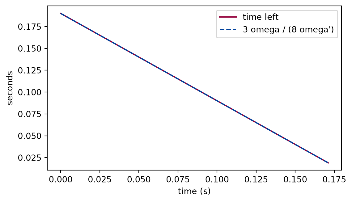
The cell integrates the shrinking orbit, with no use of the closed form, and computes $3\omega/(8\omega')$ at each time from the frequency and the rate. The theorem says the result falls with the slope $-1$ .

def countdown():
    """The countdown 3 omega / (8 omega') along the integrated inspiral, and
    its slope against time."""
    tau0 = chirp.time_to_coalescence(f0, mc)
    times = np.linspace(0.0, 0.9 * tau0, 300)
    _, f_num = chirp.inspiral_frequency(times, m1, m2, f0)
    left = 3 * f_num / (8 * chirp.chirp_rate(f_num, mc))
    slope = np.polyfit(times, left, 1)[0]
    return tau0, times, left, slope

src/pbc/mechanics/experiments/chirp_law_proved.py, lines 87 to 95, read from the repository when this page was built.

def draw_countdown(tau0, times, left) -> Figure:
    """The time left and the countdown against time."""
    fig, ax = plt.subplots(figsize=(6.4, 3.6))
    ax.plot(times, tau0 - times, color="#93003a", label="time left")
    ax.plot(times, left, color="#00429d", linestyle="--", label="3 omega / (8 omega')")
    ax.set_xlabel("time (s)")
    ax.set_ylabel("seconds")
    ax.legend()
    return fig

src/pbc/mechanics/experiments/chirp_law_proved.py, lines 98 to 106, read from the repository when this page was built.

Plot of seconds against time in seconds. A straight line of slope minus one, the time left, and a dashed curve from the integrated inspiral lie on top of each other. — Figure 1: simulated The quantity 3 omega / (8 omega’) along an integrated inspiral, with the time left to coalescence. It follows the line of slope minus one.

The fitted slope is -1.0000, as the theorem says. The theorem holds wherever the law holds. Near the end of a real inspiral the law stops describing the system, and the lab says where.

Limits

Nothing about the measurement. The theorems are about equations. They do not say that the detectors saw a chirp, that the fit of the lab found the right chirp mass, or that any value of the chirp mass is correct. A proved relation between a frequency and its rate says nothing about whether the frequency and the rate were measured well.
The quadrupole power is assumed. If the true power differs, every theorem still holds as stated, but about a different system. The lesson does not derive the power from general relativity.
The Newtonian orbit. The model is the leading order. The proofs do not say how good it is near the merger, where the separation approaches the size of the black holes.
The Python code. Nothing here is a statement about pbc.mechanics.chirp. The cells above compare its output with the identities for one pair of masses.
Real numbers, differentiable motion. ℝ is exact and the motion is assumed differentiable. A numerical inspiral has a step error that the theorems do not speak about.
Only these properties. The closed form of the frequency as a function of time, and the phase of the waveform, are not proved here; the countdown theorem is the local, differential form of the closed form.

Self-check. The uniqueness theorem says a frequency and its rate fix the chirp mass. Does it say that the two masses are fixed?

With scripts, you can record in this browser that you answered this question.

Solution to the self-check

No. The chirp mass is one combination of the two masses, and many pairs $(m_1, m_2)$ give the same value of $(m_1 m_2)^3/(m_1+m_2)$ . The lab says the same: the frequency and its rate fix $\mathcal{M}$ and not the masses separately.

Exercises

Exercise 1. A different power. Suppose the orbit lost energy at a power proportional to $a^{-4}$ and not $a^{-5}$ . Which theorem of this lesson would no longer apply, and what would change in the shrink rate?

Solution to exercise 1

The shrink-rate theorem would not apply, since its hypothesis hloss states the quadrupole power. From $\tfrac{G m_1 m_2}{2a^2}\,a' = -P$ with $P \propto a^{-4}$ the rate would be proportional to $a^{-2}$ and not $a^{-3}$ , and the powers of $\omega$ in the chirp law would change with it.

def exponent_of_the_rate():
    """Exercise 1."""
    print("the exponent of a in the rate is that of the power, plus two")

src/pbc/mechanics/experiments/chirp_law_proved.py, lines 109 to 111, read from the repository when this page was built.

the exponent of a in the rate is that of the power, plus two

Exercise 2. The factor 8/3. Derive by hand that $\tau = 3\omega/(8\omega')$ falls at the rate one if $\omega' = k\,\omega^{11/3}$ .

Solution to exercise 2

$\mathrm{d}\tau/\mathrm{d}t = \tfrac38\,(\omega'^2 - \omega\omega'')/\omega'^2$ , and $\omega'' = \tfrac{11}{3}\,k\,\omega^{8/3}\omega' = \tfrac{11}{3}\,\omega'^2/\omega$ , so $\mathrm{d}\tau/\mathrm{d}t = \tfrac38\,(1 - \tfrac{11}{3}) = -1$ .

def exponent_of_the_countdown():
    """Exercise 2."""
    print(f"3/8 * (1 - 11/3) = {3 / 8 * (1 - 11 / 3):.1f}")

src/pbc/mechanics/experiments/chirp_law_proved.py, lines 114 to 116, read from the repository when this page was built.

3/8 * (1 - 11/3) = -1.0

Check this proof

This page was built from commit 6417e2ff90258bd2d2ba21d217eb7666fd24f680 of the repository.

In a clone at that commit, with the pinned Lean toolchain, this command in lean/ checks the proofs of this page:

lake build PhysicsByConstruction.Mechanics.Chirp

Files, tests, and every command

The files behind it:

site/lessons/lean/05-the-chirp-law-proved/index.qmd: this page, with every code cell.
lean/PhysicsByConstruction/Mechanics/Chirp.lean: a Lean file the page shows.
src/pbc/mechanics/chirp.py: code the experiment runs.
src/pbc/mechanics/experiments/chirp_law_proved.py: code the experiment runs.
src/pbc/experiment.py: code the experiment runs.
tests/unit/test_chirp.py: tests of that code.
tests/unit/test_chirp_law_proved_experiment.py: tests of that code.

With Git and uv, and elan for the proofs, installed (see the setup page), run:

git clone https://github.com/taspinar/physics-by-construction.git
cd physics-by-construction
git checkout 6417e2ff90258bd2d2ba21d217eb7666fd24f680
uv sync --locked --no-dev
uv run --locked --no-dev python -m pbc.mechanics.experiments.chirp_law_proved results
cd lean
lake exe cache get
lake build PhysicsByConstruction.Mechanics.Chirp

The experiment writes every figure of this page into results/, as <label>.png, and every number and table of the page, as the page shows it, into results/results.json. Its numbers match this page to the digits shown, and its figure files are the ones the page shows; digits beyond those can differ between machines, because floating-point libraries differ. Change the code of the experiment and run it again to see what changes.

lake build compiles the proofs of this page with the Lean toolchain that elan installs; the first run fetches the Mathlib build cache, which is large. The setup page says how to install elan.