Gravitational-wave strain lab

From the Kepler orbit to a chirp: the calibrated strain of the two LIGO detectors around the first detected gravitational-wave event, whitened and compared with the Newtonian-order chirp of two bodies spiralling together, and what that comparison does and does not say about the masses.

Course

Classical mechanics, lesson 13 of 28

Slot

M16, Experimental: GW150914 gravitational-wave strain

Methods

Measured data, Simulation

Difficulty

Advanced, level 3 of 3

What you’ll learn

• Derive the frequency and the rate of change of frequency of a shrinking circular orbit from Kepler’s third law and an energy loss
• Read a measured strain through the processing it needs, saying at each step what was changed
• Fit the Newtonian chirp to the whitened strain, report the chirp mass with its uncertainty, and say what the model leaves out

Prerequisites

The Kepler orbit.

Before you begin

• Complex numbers: the discrete Fourier transform of a sampled signal, its spectrum, and what a window does to it
• Statistics: a least-squares fit, the standard deviation of noise, and the chi-square of residuals

Related

The chirp law, proved

Previous

Automated analysis pipelines

Next

Inverse physics: parameters from observations

With scripts, this page keeps a record in your browser of whether you completed the lesson. Nothing is stored without them.

With scripts, this place suggests what to do next, with the reason, from the progress saved in your browser. Without them, follow the learning path.

Two black holes, each tens of times the mass of the Sun, circled each other, spiralled together, and merged, a billion years ago. The wave they sent out reached the two detectors of the Laser Interferometer Gravitational-Wave Observatory (LIGO), in Hanford and in Livingston, as a change in the distance between mirrors four kilometres apart of less than a thousandth of the width of a proton. Can the masses be read from that record with the mechanics of this course? The earlier lessons give most of the tools. The Kepler orbit gives the frequency of a circular orbit from its size, and a slow loss of energy makes the orbit shrink and the frequency rise: a chirp. The measured strain gives the rise to compare with.

The lesson goes in two directions and meets in the middle. From the orbit it derives the chirp, with one input that Newtonian mechanics does not contain, the power radiated in gravitational waves, and checks the closed form against a numerical inspiral. From the data it takes the calibrated strain of the two detectors, shows why it must be whitened before anything is visible, shows that the same signal is in both, and fits the chirp to it. The result is a number for the chirp mass with an uncertainty, set against the published value, and a statement of what a Newtonian model leaves out. Every processing step is named on the page, and every figure says whether it shows a calibrated measurement, a processed one, or a model.

Assumptions

1. Two point masses on a circular orbit. The orbit of the Kepler lesson with zero eccentricity. Gravitational radiation circularises an orbit long before the last cycles, so this is the usual case, but an orbit that starts eccentric has a different chirp.
2. Newtonian gravity for the orbit, the quadrupole formula for the loss. The orbit is the Newtonian one. The power that the pair radiates is taken from general relativity as one stated input, not derived here. Everything else follows from Newtonian mechanics, so the model is the leading order of the full theory.
3. A slow shrinking. The orbit changes little during one revolution, so at every moment it is a circle of the current radius. Near the merger this fails, and so does the Newtonian orbit itself: the lesson shows below that the separation falls under the size of the black holes.
4. The amplitude is free. The strain depends on the distance and on the orientation of the orbit, which the frequency does not, so the fit leaves the amplitude of each detector free and fixes only the shape of the chirp.
5. Noise that is the detector’s own, stationary over a few seconds. The noise spectrum is estimated from the thirty-two seconds of the sample and assumed to hold at the event. The whitened noise is then taken as independent from sample to sample with one standard deviation, which sets the uncertainty of the fit. Real detector noise has glitches and correlations, so this is the least certain assumption of the lesson.
6. The time is the catalogue time of the event. All times are seconds since the reference time of the event in the catalogue, not since the merger. The two detectors are compared with the delay measured from the data.
7. Detector frame. A signal from a distant source is stretched by the expansion of the universe, so the chirp mass the fit finds is the detector-frame one, larger than the source-frame mass by the factor one plus the redshift. The comparison below uses that factor.

From an orbit to a chirp

The frequency of a circular orbit

Two masses $m_1$ and $m_2$ on a circular orbit of separation $a$ obey the reduction of the Kepler lesson with $GM = G(m_1 + m_2)$. Kepler’s third law, $(2\pi f_\mathrm{orb})^2 a^3 = GM$, gives the orbital frequency. The wave has its strongest part at twice the orbital frequency, because the pair looks the same after half a turn, so

$$f = 2 f_\mathrm{orb} = \frac{1}{\pi}\sqrt{\frac{GM}{a^3}} .$$

An orbit that shrinks

The energy of the circular orbit is $E = -G m_1 m_2 / (2a)$. If the pair radiates the power $P = \tfrac{32}{5} G^4 m_1^2 m_2^2 M / (c^5 a^5)$ of the quadrupole formula, the energy falls at that rate and the separation follows,

$$\frac{\mathrm{d}a}{\mathrm{d}t} = -\frac{64}{5}\,\frac{G^3 m_1 m_2 M}{c^5 a^3},$$

so the orbit shrinks ever faster as it shrinks. Writing $a$ as a function of $f$ with the equation above and differentiating gives the rate of change of the frequency,

$$\frac{\mathrm{d}f}{\mathrm{d}t} = \frac{96}{5}\,\pi^{8/3}\left(\frac{G\mathcal{M}}{c^3}\right)^{5/3} f^{11/3}, \qquad \mathcal{M} = \frac{(m_1 m_2)^{3/5}}{(m_1 + m_2)^{1/5}} .$$

The masses enter only through the chirp mass $\mathcal{M}$. That is why a measurement of the frequency and of its rate fixes this one combination and not the two masses separately. Integrating the equation gives the frequency before the coalescence time $t_c$, where it would diverge,

$$f(t) = \frac{1}{\pi}\left(\frac{5}{256\,(t_c - t)}\right)^{3/8} \left(\frac{G\mathcal{M}}{c^3}\right)^{-5/8},$$

and, solved the other way, the chirp mass from a frequency and its rate: $G\mathcal{M}/c^3 = \bigl(\tfrac{5}{96}\pi^{-8/3} f^{-11/3}\dot f\bigr)^{3/5}$. The wave itself is $h(t) \propto f^{2/3} \cos\varphi(t)$ with the phase $\varphi = -2\,\bigl((t_c - t)/(5G\mathcal{M}/c^3)\bigr)^{5/8}$ plus a constant; the amplitude scale is free.

Checking the closed form

The closed form follows from a chain of algebra, and a chain of algebra can hide a slip. The cell below integrates the shrinking separation numerically, with no use of the closed form, for two bodies of the mass of the first published estimate, and compares the frequency along the way.

m1, m2, f_start = 36.0, 29.0, 35.0  # solar masses, Hz: given values of the example

src/pbc/mechanics/experiments/gravitational_wave_strain.py, line 55, read from the repository when this page was built.

def inspiral_check(experiment: Experiment):
    """The inspiral integrated numerically against the closed form, and the
    orbit at the start through the orbit module of the Kepler lesson;
    record the table and return the largest relative difference, the
    frequency of the orbit, in Hz, and the rows."""
    mc_example = chirp.chirp_mass(m1, m2)
    tau0 = chirp.time_to_coalescence(f_start, mc_example)
    times = np.linspace(0.0, 0.95 * tau0, 400)
    _, f_numeric = chirp.inspiral_frequency(times, m1, m2, f_start)
    f_closed = chirp.chirp_frequency(times, mc_example, tau0)
    worst = float(np.max(np.abs(f_numeric / f_closed - 1.0)))

    # The orbit at the start, through the orbit module of the Kepler lesson.
    a0 = float(chirp.separation_from_frequency(f_start, m1 + m2))
    gm_total = (m1 + m2) * chirp.GM_SUN
    start = State(0.0, np.array([a0, 0.0]), np.array([0.0, np.sqrt(gm_total / a0)]))
    orbit = orbital_elements(start, gm_total)
    f_from_orbit = 2.0 / orbit.period

    rows = []
    for fraction in (0.0, 0.5, 0.9, 0.95):
        k = min(round(fraction * (len(times) - 1) / 0.95), len(times) - 1)
        a_k = float(chirp.separation_from_frequency(f_numeric[k], m1 + m2))
        rows.append((times[k], f_numeric[k], f_closed[k], a_k / 1e3))
    experiment.table(
        "inspiral-check",
        rows,
        columns=[
            ("time", "s", ".3f"),
            ("frequency, integrated orbit", "Hz", ".1f"),
            ("frequency, closed form", "Hz", ".1f"),
            ("separation", "km", ".0f"),
        ],
        caption="The inspiral of two bodies integrated numerically and from the "
        "closed form.",
    )
    return worst, f_from_orbit, rows

src/pbc/mechanics/experiments/gravitational_wave_strain.py, lines 65 to 101, read from the repository when this page was built.

The inspiral of two bodies integrated numerically and from the closed form.

time (s)	frequency, integrated orbit (Hz)	frequency, closed form (Hz)	separation (km)
0.000	35.0	35.0	894
0.095	45.4	45.4	751
0.171	83.0	83.0	502
0.181	107.6	107.6	423

Numerically verified (circular orbit, leading order, the example masses): The frequency of the integrated inspiral and the closed form agree to 3e-08 in relative terms over the first 95 percent of the time to coalescence, and the frequency of the starting orbit from orbital_elements is 35.0 Hz, as it was set. The separation in the last column ends near 423 km, while the horizon of a black hole of the total mass has a radius of 192 km. A Newtonian orbit of two bodies cannot be trusted once the separation is a few times that radius, which is why the comparison with data below stops before the merger.

The program

The functions are short, and the page shows the two that carry the physics.

def chirp_frequency(t: ArrayLike, mc: float, t_c: float) -> Array:
    """Wave frequency in hertz at time ``t`` for chirp mass ``mc`` (solar masses).

    ``f = (1 / pi) (5 / (256 tau))^(3/8) (G Mc / c^3)^(-5/8)`` with the time to
    coalescence ``tau = t_c - t``. It diverges at ``t_c``, where the Newtonian
    orbit has long stopped being a good model; times at or after ``t_c`` give
    ``nan``.
    """
    tau = t_c - np.asarray(t, dtype=float)
    with np.errstate(invalid="ignore", divide="ignore"):
        f = (5.0 / (256.0 * tau)) ** 0.375 / (np.pi * (mc * GM_SUN_OVER_C3) ** 0.625)
    return np.where(tau > 0, f, np.nan)

src/pbc/mechanics/chirp.py, lines 63 to 74, read from the repository when this page was built.

def chirp_mass_from_rate(f: ArrayLike, fdot: ArrayLike) -> Array:
    """Chirp mass in solar masses from a frequency and its rate of change.

    The inverse of ``chirp_rate``:
    ``G Mc / c^3 = ((5/96) pi^(-8/3) f^(-11/3) fdot)^(3/5)``.
    """
    f = np.asarray(f, dtype=float)
    fdot = np.asarray(fdot, dtype=float)
    return (
        (5.0 / 96.0) * np.pi ** (-8.0 / 3.0) * f ** (-11.0 / 3.0) * fdot
    ) ** 0.6 / GM_SUN_OVER_C3

src/pbc/mechanics/chirp.py, lines 100 to 110, read from the repository when this page was built.

Worked examples

The measured strain

Data card

Dataset

GW150914 gravitational-wave strain, H1 and L1, 32 s at 4096 Hz

Source

https://gwosc.org/events/GW150914/, DOI https://doi.org/10.7935/82H3-HH23, LIGO Scientific Collaboration and Virgo Collaboration, distributed by the Gravitational Wave Open Science Center (GWOSC); GWTC-1-confident, GW150914 v3, strain release R1

Licence

CC-BY-4.0

Attribution

Data: GWOSC, GW150914 v3, CC BY 4.0; whitened, band-passed and fitted here (changes indicated on each figure). Data-release paper: R. Abbott et al. (LIGO Scientific Collaboration and Virgo Collaboration), "Open data from the first and second observing runs of Advanced LIGO and Advanced Virgo", SoftwareX 13 (2021) 100658. Acknowledgement (https://gwosc.org/acknowledgement/, read 2026-10-11): "This research has made use of data or software obtained from the Gravitational Wave Open Science Center (gwosc.org), a service of the LIGO Scientific Collaboration, the Virgo Collaboration, and KAGRA. This material is based upon work supported by NSF's LIGO Laboratory which is a major facility fully funded by the National Science Foundation, as well as the Science and Technology Facilities Council (STFC) of the United Kingdom, the Max-Planck-Society (MPS), and the State of Niedersachsen/Germany for support of the construction of Advanced LIGO and construction and operation of the GEO600 detector. Additional support for Advanced LIGO was provided by the Australian Research Council. Virgo is funded, through the European Gravitational Observatory (EGO), by the French Centre National de Recherche Scientifique (CNRS), the Italian Istituto Nazionale di Fisica Nucleare (INFN) and the Dutch Nikhef, with contributions by institutions from Belgium, Germany, Greece, Hungary, Ireland, Japan, Monaco, Poland, Portugal, Spain. KAGRA is supported by Ministry of Education, Culture, Sports, Science and Technology (MEXT), Japan Society for the Promotion of Science (JSPS) in Japan; National Research Foundation (NRF) and Ministry of Science and ICT (MSIT) in Korea; Academia Sinica (AS) and National Science and Technology Council (NSTC) in Taiwan."

Calibration

Strain is calibrated by the LIGO calibration pipeline before release; the plain-text product states no calibration uncertainty. The GWOSC event page and the data-release papers document it; this spike did not verify it.

Masks

None in the files: no NaN, no data-quality flags in the text product (the HDF5 product carries them).

Uncertainty

No per-sample uncertainty is released; the noise is the data's own spectrum, estimated from the 32 s (Welch).

Artifacts of the dataset GW150914 gravitational-wave strain, H1 and L1, 32 s at 4096 Hz and the figure status each gives

Artifact	Type	Figure status	What it is
H-H1_GWOSC_4KHZ_R1-1126259447-32.txt.gz	calibrated-observation	calibrated	Calibrated strain h(t) of the LIGO Hanford detector, as released by GWOSC; instrument noise included, no signal subtracted.
L-L1_GWOSC_4KHZ_R1-1126259447-32.txt.gz	calibrated-observation	calibrated	Calibrated strain h(t) of the LIGO Livingston detector.
whitened, band-passed strain (derived by pbc.data.reference.gw150914)	calibrated-observation	calibrated	Not a data file: the figure's processed series. Filtering is disclosed on the figure; it is labelled processed there.

A sample is committed in data/samples/gw150914-strain/; the figures on this page are made from it.

The full data: ./scripts/fetch-data.sh gw150914-strain downloads it into data/downloads/ and checks its digest. The site build and the checks never download anything.

No-LLM path. Everything on this page, the figures included, is reproduced from the files named here by the code of the page, with no language model and no account. An agent may help you explore the data; what it says is never data.

The two files hold the calibrated strain $h(t)$ of each detector, thirty-two seconds at 4096 samples per second, exactly as GWOSC released them. They are calibrated observations: the output of the calibration pipeline of LIGO, not a raw detector channel, and the file states no per-sample uncertainty. The data are released under a Creative Commons attribution licence; the card above gives the data-release paper to cite and the full acknowledgement, with its funding text, and both apply to every figure of this page.

def load_strain():
    """The strain of both detectors from the committed sample, with the raw
    RMS of each."""
    strains = {
        name: read_strain(SAMPLES_DIR / "gw150914-strain" / file)
        for name, file in FILES.items()
    }
    assert all(
        s.event.startswith("GW150914") and s.sample_rate == 4096.0
        for s in strains.values()
    )
    raw_rms = {name: float(np.std(s.strain)) for name, s in strains.items()}
    return strains, raw_rms

src/pbc/mechanics/experiments/gravitational_wave_strain.py, lines 104 to 116, read from the repository when this page was built.

def draw_calibrated_strain(strains) -> Figure:
    """Four seconds of the calibrated strain and the noise spectrum."""
    segments = {name: cut_segment(s) for name, s in strains.items()}
    fig, (top, bottom) = plt.subplots(2, 1, figsize=(7.2, 6.2), constrained_layout=True)
    for k, (name, seg) in enumerate(segments.items()):
        top.plot(
            seg.time, seg.strain * 1e19, lw=0.6, color=FIGURE_COLOURS[k], label=name
        )
        freqs, asd = amplitude_spectrum(strains[name])
        bottom.loglog(freqs[1:], asd[1:], lw=0.9, color=FIGURE_COLOURS[k], label=name)
    top.set_xlabel("time since the event [s]")
    top.set_ylabel("strain, calibrated [1e-19]")
    top.set_title("Calibrated strain of the two detectors, four seconds")
    top.legend(loc="upper right")
    bottom.set_xlim(10, 2000)
    bottom.set_xlabel("frequency [Hz]")
    bottom.set_ylabel("amplitude spectral density [1/sqrt(Hz)]")
    bottom.set_title("Noise spectrum: Welch estimate over the whole file (processed)")
    bottom.legend(loc="upper right")
    label_status(fig, "calibrated")
    add_credit(
        fig, "Data: GWOSC, GW150914 v3, CC BY 4.0. Spectrum: processed from the strain."
    )
    return fig

src/pbc/mechanics/experiments/gravitational_wave_strain.py, lines 119 to 142, read from the repository when this page was built.

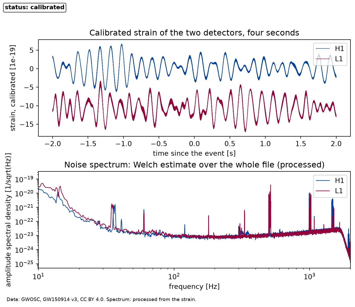
Figure 1: calibrated Calibrated strain of the two detectors in the four seconds around the event, and the amplitude spectrum of the noise of each. The event is not visible by eye: the strain is dominated by noise at low frequency.

The upper panel is the calibrated strain itself. Its rms is about 2.2 in units of $10^{-19}$ in Hanford, and nothing like a chirp can be seen. The lower panel is why: the noise is orders of magnitude larger at low frequency than near the best frequencies of the detector, so the strain is a sum dominated by slow wandering, and the signal sits in the band where the noise is smallest. The spectrum of the lower panel is an estimate, the Welch average of overlapping stretches of four seconds over the whole file, and the figure labels it processed.

Whitening, and what it changes

Whitening divides the spectrum of the strain by this noise spectrum, so that every frequency has the same noise level, and a band-pass keeps the band where the detector can hear. Both operations are linear filters. They change the data: the whitened series is a processed series, the amplitudes are in units of the noise and not in units of strain, and a feature in it is only as real as the noise estimate. The cell applies them to the four seconds around the event and measures the noise of one whitened sample away from the event.

BAND = (35.0, 350.0)  # Hz, the band of the primary analysis

src/pbc/mechanics/experiments/gravitational_wave_strain.py, line 58, read from the repository when this page was built.

def whitened(strains):
    """Two seconds around the event, whitened and band-passed, the noise in
    these units, and the processing steps as the figures disclose them."""
    duration = strains["H1"].duration
    big = {name: cut_segment(s, 2.0) for name, s in strains.items()}
    whiteners_big = {
        name: make_whitener(strains[name], big[name], BAND) for name in strains
    }
    white_big = {name: whiteners_big[name](big[name].strain) for name in strains}
    time_big = big["H1"].time
    sigma_big = noise_sigma(white_big["H1"], time_big, (0.5, 1.6))
    steps = ("whitened", f"band-passed {BAND[0]:g} to {BAND[1]:g} Hz")
    steps_long = (
        f"whitened by the Welch spectrum of the {duration:g} s file, "
        f"band-passed {BAND[0]:g} to {BAND[1]:g} Hz, "
        "cut to the seconds around the event"
    )
    return big, white_big, time_big, sigma_big, steps, steps_long

src/pbc/mechanics/experiments/gravitational_wave_strain.py, lines 145 to 162, read from the repository when this page was built.

The steps are, in order: whitened by the Welch spectrum of the 32 s file, band-passed 35 to 350 Hz, cut to the seconds around the event. A whitened sample away from the event has a standard deviation of 0.38 in these units, which is the uncertainty that the fit below uses for one sample.

One signal in two detectors

Before any model, the data can say whether the same thing happened at the two sites. The sites are about three thousand kilometres apart, so a wave at the speed of light reaches them within ten milliseconds of each other. The cell correlates the whitened Hanford series with the Livingston one over a window of a fifth of a second around the event, searching the delay within that limit and allowing either sign. It then repeats exactly the same procedure on the windows away from the event, to see what chance gives.

def detector_correlation(white_big, time_big, rate):
    """The correlation of the two detectors and of quiet control windows."""
    corr = correlation_with_control(white_big["H1"], white_big["L1"], time_big, rate)
    control_max = float(corr["controls"].max())
    lag_ms = 1e3 * corr["lag"]
    return corr, control_max, lag_ms

src/pbc/mechanics/experiments/gravitational_wave_strain.py, lines 165 to 170, read from the repository when this page was built.

Observational (whitened and band-passed strain, windows of a fifth of a second, delay searched within the light travel time): The whitened strains of the two detectors correlate at the event with a coefficient of magnitude 0.71 at a delay of 7.3 milliseconds, with the sign reversed and the Livingston detector first. The same procedure on the 8 quiet windows of the segment never gives more than 0.23. The delay is inside the light travel time, as a signal from space requires, and the negative sign says that the two detectors, which are rotated against each other, answer with opposite signs. No model is needed for this statement. It does not say what produced the signal, nor how significant it is beyond the number of control windows: the published significance of the detection is a result of the collaboration, obtained with a far larger set of control data, and is not reproduced here.

Time and frequency

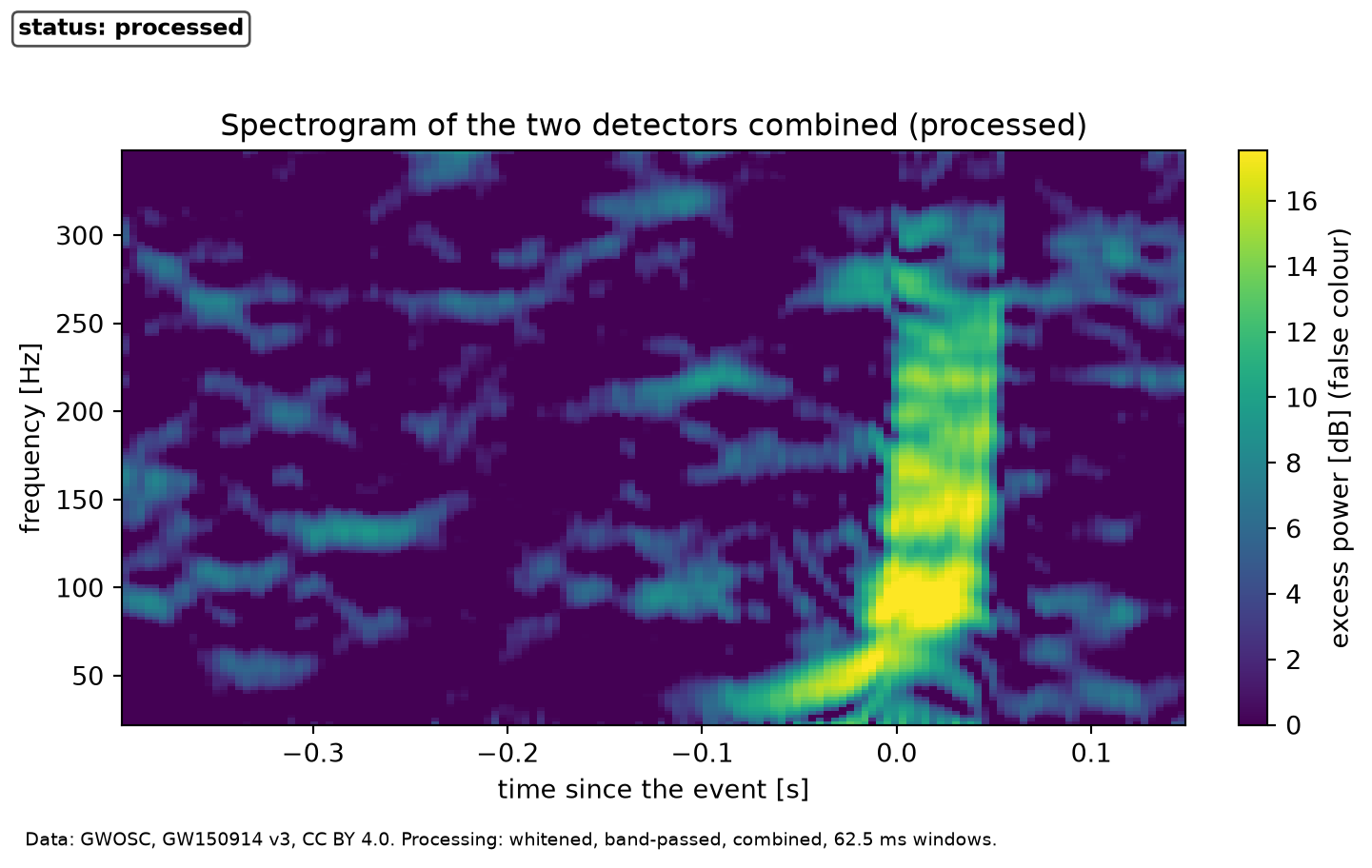
A chirp is a signal whose frequency changes in time, and a spectrogram shows that: the spectrum of short stretches, one beside the next. The detectors are combined for this figure: the Livingston series is shifted by the measured delay and, given the negative correlation, inverted, and subtracted from the Hanford one, so that the signal adds and the independent noise adds less.

def spectrogram_data(big, white_big, corr, rate):
    """The spectrogram of the two detectors combined, as excess power over
    the median before the event, in dB."""
    shift = round(corr["lag"] * rate)
    sign = -1.0 if corr["correlation"] < 0 else 1.0
    combined = white_big["H1"] + sign * np.roll(white_big["L1"], -shift)
    n_window = 256
    f_grid, t_grid, power = sp_signal.spectrogram(
        combined, rate, nperseg=n_window, noverlap=n_window - 16, nfft=2048
    )
    t_grid = t_grid + big["H1"].time[0]
    shown_t = (t_grid > -0.4) & (t_grid < 0.15)
    shown_f = (f_grid > 20) & (f_grid < 350)
    excess = 10 * np.log10(
        power[np.ix_(shown_f, shown_t)]
        / np.median(power[shown_f][:, t_grid < -0.5], axis=1)[:, None]
    )
    window_length = n_window / rate
    frequency_width = 1.0 / window_length
    return (
        f_grid,
        t_grid,
        power,
        shown_t,
        shown_f,
        excess,
        window_length,
        frequency_width,
    )

src/pbc/mechanics/experiments/gravitational_wave_strain.py, lines 173 to 201, read from the repository when this page was built.

The time-frequency picture has a built-in limit. Each column is the spectrum of 62.5 milliseconds of data, so its frequencies are resolved only to about 16 hertz, and a feature shorter than that window is smeared in time. A longer window would sharpen the frequency and blur the time; the product of the two widths is about one. The window is part of what is shown, and the page fixes it.

def draw_spectrogram(f_grid, t_grid, shown_t, shown_f, excess) -> Figure:
    """The spectrogram of the two detectors combined."""
    fig, ax = plt.subplots(figsize=(7.4, 4.6), constrained_layout=True)
    extent = (
        t_grid[shown_t][0],
        t_grid[shown_t][-1],
        f_grid[shown_f][0],
        f_grid[shown_f][-1],
    )
    sequential_image(
        ax,
        excess,
        label="excess power",
        unit="dB",
        extent=extent,
        aspect="auto",
        vmin=0,
        vmax=np.percentile(excess, 99.5),
    )
    ax.set_xlabel("time since the event [s]")
    ax.set_ylabel("frequency [Hz]")
    ax.set_title("Spectrogram of the two detectors combined (processed)")
    label_status(fig, "processed")
    add_credit(
        fig,
        "Data: GWOSC, GW150914 v3, CC BY 4.0. Processing: whitened, band-passed,"
        " combined, 62.5 ms windows.",
    )
    return fig

src/pbc/mechanics/experiments/gravitational_wave_strain.py, lines 204 to 232, read from the repository when this page was built.

Figure 2: processed Excess power of the two detectors combined, in decibels above the noise at each frequency, against time and frequency. A bright track rises in frequency in the last tenth of a second before the event time, followed by a broad band at all frequencies. The colours are false colour.

A figure of this kind is a still of something that moves, and the page does not depend on any animation: the track is the whole content. Read the colour scale as the power of each cell compared with the power the same frequency has in the quiet half second before; it is a false colour, chosen to be readable, and not the colour of anything. The table after the fit lists the frequency of the strongest cell at several times, with the frequency of the model beside it.

Fitting the Newtonian chirp

The fit uses the model of the first section. The chirp mass and the coalescence time are shared by the two detectors; each detector has its own amplitude and phase, as two linear coefficients, and its own arrival time, the measured delay. The model is passed through the same whitening as the data, so the comparison is made in the whitened domain, with the chi-square of the residuals over the noise of one sample. The window of the primary analysis runs from two tenths of a second before the event time to the event time, which ends before the model’s frequency has reached the value where the Newtonian orbit has stopped being credible.

PRIMARY_WINDOW = (-0.2, 0.0)

src/pbc/mechanics/experiments/gravitational_wave_strain.py, line 61, read from the repository when this page was built.

def analyse(strains, seg, corr, band, window, step=1.0, span=(22.0, 50.0)):
    """Fit the Newtonian chirp to both detectors in a band and a window."""
    time_fit = seg["H1"].time
    whiteners = {
        name: make_whitener(strains[name], seg[name], band) for name in strains
    }
    data = {name: whiteners[name](seg[name].strain) for name in strains}
    sigma = noise_sigma(data["H1"], time_fit, (0.3, 0.65))
    result = fit_chirp(
        time_fit,
        data,
        whiteners,
        {"H1": 0.0, "L1": corr["lag"]},
        window=window,
        sigma=sigma,
        mc_grid=np.arange(span[0], span[1], step),
    )
    return result, data, sigma

src/pbc/mechanics/experiments/gravitational_wave_strain.py, lines 235 to 252, read from the repository when this page was built.

def primary_fit(strains, corr):
    """The fit of the primary band and window, and the frequency and its rate
    of the fitted chirp at the ends of the window."""
    seg = {name: cut_segment(s, 0.75) for name, s in strains.items()}
    primary, data_fit, sigma_fit = analyse(strains, seg, corr, BAND, PRIMARY_WINDOW)
    mc_fit = primary.mc
    f_at_end = float(chirp.chirp_frequency(PRIMARY_WINDOW[1], mc_fit, primary.t_c))
    f_at_start = float(chirp.chirp_frequency(PRIMARY_WINDOW[0], mc_fit, primary.t_c))
    fdot_at_end = float(chirp.chirp_rate(f_at_end, mc_fit))
    check_mc = float(chirp.chirp_mass_from_rate(f_at_end, fdot_at_end))
    return (
        seg,
        primary,
        data_fit,
        sigma_fit,
        f_at_start,
        f_at_end,
        fdot_at_end,
        check_mc,
    )

src/pbc/mechanics/experiments/gravitational_wave_strain.py, lines 255 to 274, read from the repository when this page was built.

def measured_and_model(seg, primary, data_fit, sigma_fit, steps):
    """The whitened Hanford strain around the event and the fitted model, as
    series that disclose what they are."""
    time_fit = seg["H1"].time
    show = (time_fit > -0.25) & (time_fit < 0.05)
    measured = Series(
        x=time_fit[show],
        y=data_fit["H1"][show],
        sigma=np.full(show.sum(), sigma_fit),
        artifact="calibrated-observation",
        steps=steps,
        x_name="time since the event",
        x_unit="s",
        y_name="whitened strain",
        y_unit="1",
    )
    model = Series(
        x=time_fit[show],
        y=primary.models["H1"][show],
        artifact="synthetic-test",
        x_name="time since the event",
        x_unit="s",
        y_name="whitened strain",
        y_unit="1",
    )
    return measured, model

src/pbc/mechanics/experiments/gravitational_wave_strain.py, lines 277 to 302, read from the repository when this page was built.

def draw_measured_vs_model(measured, model) -> Figure:
    """The measured strain against the fitted chirp, with the residuals."""
    fig, _ = measured_vs_model(
        measured,
        {"Newtonian chirp (fitted)": model},
        window=PRIMARY_WINDOW,
        figsize=(8.6, 6.0),
    )
    add_credit(
        fig,
        "Data: GWOSC, GW150914 v3, CC BY 4.0. Hanford detector, whitened and"
        " band-passed; model whitened the same way.",
    )
    check_figure(fig, residuals=True)
    return fig

src/pbc/mechanics/experiments/gravitational_wave_strain.py, lines 305 to 319, read from the repository when this page was built.

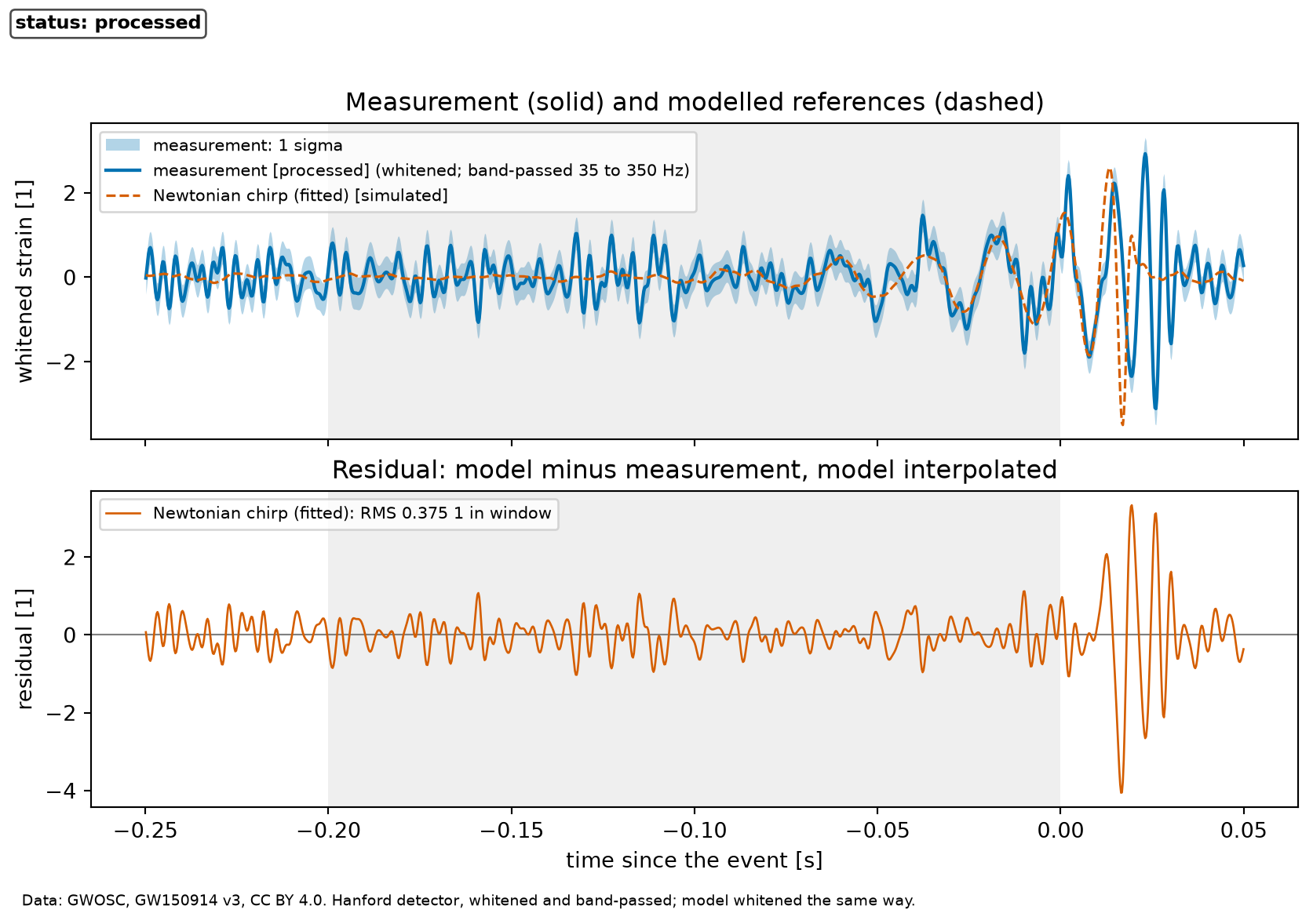
Figure 3: processed The whitened Hanford strain (solid, with one standard deviation of the noise as a band) and the fitted Newtonian chirp (dashed) around the event, with the residuals below. The model is a fit to the data in the shaded window and is drawn apart from it.

With scripts, a button below the figure loads the whitened strain and the best chirp of a range of chirp masses, and a slider moves between them with the error metrics of each. Without scripts the figure shows the best fit, and the profile figure further down gives the chi-square of the others.

The solid curve is the whitened measurement, and every step that produced it is named: whitened; band-passed 35 to 350 Hz. The dashed curve is the model, a fit and not a measurement, drawn apart. Inside the shaded window the model follows the oscillations of the data and the residual shows no structure at the scale of the noise. The reduced chi-square of the fit is 0.85 for 1638 samples of both detectors, as it should be near one if the model and the noise estimate describe the data. Outside the window, after the event time, the model is not fitted and the data go on with a signal that the Newtonian model cannot describe.

'index_files/figure-html/chirp-masses.json'

The spectrogram can be checked against the fitted model in frequency as well: the table lists, for a few times, the frequency of the strongest cell of the spectrogram below two hundred hertz and the frequency the fitted chirp has then. It is also the text alternative of the spectrogram figure.

def ridge_table(experiment: Experiment, f_grid, t_grid, power, primary) -> None:
    """The strongest spectrogram cell against the fitted chirp at six times;
    record the table."""
    ridge_times = [-0.06, -0.05, -0.04, -0.03, -0.02, -0.01]
    low = f_grid < 200
    rows = []
    for moment in ridge_times:
        column = int(np.argmin(np.abs(t_grid - moment)))
        strongest = float(f_grid[low][np.argmax(power[low, column])])
        rows.append(
            (
                moment,
                strongest,
                float(chirp.chirp_frequency(moment, primary.mc, primary.t_c)),
            )
        )
    experiment.table(
        "ridge-table",
        rows,
        columns=[
            ("time since the event", "s", ".2f"),
            ("strongest cell of the spectrogram", "Hz", ".0f"),
            ("fitted chirp", "Hz", ".0f"),
        ],
        caption="The frequency of the strongest spectrogram cell and of the fitted "
        "Newtonian chirp at six times before the event.",
    )

src/pbc/mechanics/experiments/gravitational_wave_strain.py, lines 356 to 382, read from the repository when this page was built.

The frequency of the strongest spectrogram cell and of the fitted Newtonian chirp at six times before the event.

time since the event (s)	strongest cell of the spectrogram (Hz)	fitted chirp (Hz)
-0.06	40	38
-0.05	42	40
-0.04	44	43
-0.03	48	46
-0.02	52	50
-0.01	58	56

The strongest cell follows the model where the signal is strongest, close to the event, and the resolution of the window, about sixteen hertz, is the difference to expect. Earlier than that the signal is below the noise in a single cell and the strongest cell is a noise peak, which is why the fit uses the whole waveform and not a track of the spectrogram.

The chirp mass, and how sure it is

The fit gives a chirp mass of 41.0 solar masses, with the coalescence time 19 milliseconds after the event time. The model’s frequency runs from 26 hertz (under the lower edge of the band) at the start of the window to 66 hertz at its end, with a rate of change of 1322 hertz per second there; turned back into a mass with the inversion formula, that frequency and rate give 41.0 solar masses again, which is the same statement in the other direction.

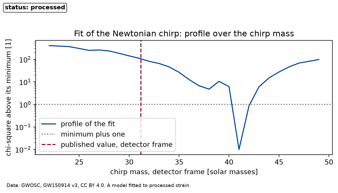
The uncertainty has two parts. The first is statistical: the profile of the chi-square over the chirp mass, with the coalescence time minimised at each mass, which the figure below draws. The interval where it stays within one of its minimum is 40.8 to 42.0 solar masses. The fit helper fit_curve of the course also reports whether the data tell the parameters apart, and the next cell prints what it says for this fit. The chirp mass and the coalescence time are tied, because a heavier chirp that coalesces later looks similar over a short window, and the printed ratio of the smallest to the largest singular value of the scaled Jacobian measures how tied: the helper calls a combination undetermined below 1e-04.

def fit_diagnostics(primary):
    """The warnings of the fit and the conditioning of its Jacobian."""
    fit_warnings = primary.fit.warnings
    singular_ratio = primary.fit.singular_ratio
    print("fit warnings:", "; ".join(fit_warnings) if fit_warnings else "none")
    print(
        "smallest over largest singular value of the scaled Jacobian:"
        f" {singular_ratio:.1e}"
    )

src/pbc/mechanics/experiments/gravitational_wave_strain.py, lines 385 to 393, read from the repository when this page was built.

fit warnings: the data do not determine chirp mass separately (a combination of them is not constrained)
smallest over largest singular value of the scaled Jacobian: 1.6e-05

The second part is the choice of analysis. The cell below repeats the whole fit with three bands and with three windows, changing one choice at a time, and the table shows how much the number moves. A row where the best coalescence time runs to the end of the search is not a result, and is marked.

def sensitivity(experiment: Experiment, strains, seg, corr, primary):
    """The best chirp mass for each choice of band and window; record the
    table and return the spread of the usable results."""
    bands = [(35.0, 350.0), (35.0, 250.0), (30.0, 300.0)]
    windows = [(-0.2, 0.0), (-0.15, 0.0), (-0.2, -0.01)]
    rows, usable = [], []
    choices = [(band, windows[0]) for band in bands] + [
        (bands[0], window) for window in windows[1:]
    ]
    for band, window in choices:
        # The first choice is the fit above; it is not computed a second time.
        if (band, window) == (BAND, PRIMARY_WINDOW):
            result = primary
        else:
            result, _, _ = analyse(
                strains, seg, corr, band, window, step=2.0, span=(26.0, 48.0)
            )
        rows.append(
            (
                f"{band[0]:g} to {band[1]:g}",
                f"{window[0]:g} to {window[1]:g}",
                result.mc,
                result.t_c * 1e3,
                "end of the search: not a result" if result.at_edge else "",
            )
        )
        if not result.at_edge:
            usable.append(result.mc)
    spread = (min(usable), max(usable))
    experiment.table(
        "sensitivity",
        rows,
        columns=[
            ("band", "Hz", "s"),
            ("window", "s", "s"),
            ("chirp mass", "solar masses", ".1f"),
            ("coalescence time", "ms", ".0f"),
            ("note", "", "s"),
        ],
        caption="Best chirp mass for each choice of band and window of the fit. "
        "The first row is the fit above; the other rows search a grid of masses "
        "with a step of two solar masses.",
    )
    return spread

src/pbc/mechanics/experiments/gravitational_wave_strain.py, lines 396 to 439, read from the repository when this page was built.

Best chirp mass for each choice of band and window of the fit. The first row is the fit above; the other rows search a grid of masses with a step of two solar masses.

band (Hz)	window (s)	chirp mass (solar masses)	coalescence time (ms)	note
35 to 350	-0.2 to 0	41.0	19
35 to 250	-0.2 to 0	37.8	25
30 to 300	-0.2 to 0	41.4	19
35 to 350	-0.15 to 0	36.4	27
35 to 350	-0.2 to -0.01	41.6	18

def draw_profile(primary, published_detector) -> Figure:
    """The profile of the chi-square over the chirp mass."""
    fig, ax = plt.subplots(figsize=(6.8, 3.8), constrained_layout=True)
    delta = primary.profile_chi2 - primary.profile_chi2.min()
    ax.semilogy(
        primary.profile_mc,
        np.maximum(delta, 1e-2),
        color=FIGURE_COLOURS[0],
        label="profile of the fit",
    )
    ax.axhline(1.0, color="0.4", linestyle=":", label="minimum plus one")
    ax.axvline(
        published_detector,
        color=FIGURE_COLOURS[1],
        linestyle="--",
        label="published value, detector frame",
    )
    ax.set_xlabel("chirp mass, detector frame [solar masses]")
    ax.set_ylabel("chi-square above its minimum [1]")
    ax.set_title("Fit of the Newtonian chirp: profile over the chirp mass")
    ax.legend()
    label_status(fig, "processed")
    add_credit(
        fig, "Data: GWOSC, GW150914 v3, CC BY 4.0. A model fitted to processed strain."
    )
    return fig

src/pbc/mechanics/experiments/gravitational_wave_strain.py, lines 442 to 467, read from the repository when this page was built.

Figure 4: processed The chi-square of the fit over the chirp mass, minimised over the coalescence time at each mass, relative to its minimum. The dotted line marks one above the minimum, and the dashed vertical line the published value, shifted to the detector frame.

The statistical interval is narrow, because the noise is taken as white and the model as exact, and neither is true. The spread over the choices of the table, from 36 to 42 solar masses, is the honest size of the uncertainty of this method, and it is several times the statistical interval.

Against the published value

    ratio = mc_fit / published_detector

src/pbc/mechanics/experiments/gravitational_wave_strain.py, line 576, read from the repository when this page was built.

The collaboration publishes a chirp mass in the source frame of 28.6 solar masses for this event, and a redshift of 0.09. In the detector frame that is 31.2 solar masses. Observational (as quoted, source frame): The published chirp mass of this event is quoted from the GWOSC record of the event, in the source frame, with its redshift.

Experimentally supported (Newtonian-order model, window ending before the merger, white-noise assumption): The fit of the Newtonian chirp to the measured strain gives a detector-frame chirp mass of 41 solar masses, with a statistical interval of 40.8 to 42.0 and a spread of 36 to 42 over the analysis choices. It is 32 percent above the published value. The simplified Newtonian fit gives a chirp mass substantially higher than the published value. This discrepancy shows the limits of the model and of the analysis method. The published value comes from waveforms with higher-order terms that this model lacks, and the processing, the method of the fit, and the assumptions of the model can each contribute as well; the results of this lesson do not show how much each of them does. The statistical interval and the spread over the analysis choices do not capture the full systematic uncertainty. The lab demonstrates the underlying physics, and should not be read as a precision measurement.

Limits

What the Newtonian model does not capture: it is the leading order of the full theory and misses the following.

• Higher-order corrections. The speed of the bodies is a sizeable fraction of the speed of light in the last cycles, and the corrections in powers of that speed change the phase. They can contribute to the difference above; this lesson does not separate their effect from that of the processing and of the fit. The published masses come from waveforms that include them.
• The merger and the ringdown. After the event time the signal is the collision and the settling of the final black hole, which no Newtonian orbit describes: the separation of the example falls below the size of the horizon. The fit window stops before.
• The two masses separately. The chirp mass is one combination. The ratio of the masses enters through the next order and through the spins, and the data of this lesson do not constrain it.
• The processing. A whitened series depends on the noise estimate, the band, and the window, and the table above shows that dependence as a spread of the result. Whitening is not a measurement; the statement of the chirp mass is an inference through the model, not a reading of the data.
• The noise. Real noise has glitches and is not white after whitening, so the statistical interval is too small. The significance of the detection is not claimed here, beyond the published one.
• The frame. The mass is in the detector frame; the source-frame mass needs the distance, which the frequency does not give.

In plain words: two detectors three thousand kilometres apart recorded the same rising tone, a fraction of a second long, and a Newtonian picture of two bodies spiralling together reproduces how fast it rises and puts the one combination of the two masses that sets the rise at a few tens of times the mass of the Sun. The picture is good to within the spread of the table and fails where the bodies touch.

Self-check. The fit gives the chirp mass, not the two masses. What would you have to measure besides the frequency and its rate to get each mass, and why does the leading-order chirp not give it?

With scripts, you can record in this browser that you answered this question.

Solution to the self-check

At leading order the frequency and its rate depend on the masses only through the chirp mass, so every pair of masses with the same chirp mass gives the same chirp. Separating them needs a quantity that depends on the mass ratio: the next-order correction to the rise of the frequency, or the amplitude of the strain at a known distance, or the ringdown after the merger.

Exercises

Exercise 1. Mass from a frequency and a rate. A chirp passes $60$ Hz with a rate of change of $120$ Hz/s. What chirp mass does the Newtonian model assign to it?

Solution to exercise 1

The inversion formula applies directly.

def mass_from_a_rate():
    """Exercise 1: the chirp mass of a signal at 60 Hz rising by 120 Hz/s."""
    exercise_mc = float(chirp.chirp_mass_from_rate(60.0, 120.0))
    print(f"chirp mass: {exercise_mc:.1f} solar masses")

src/pbc/mechanics/experiments/gravitational_wave_strain.py, lines 470 to 473, read from the repository when this page was built.

chirp mass: 12.0 solar masses

Exercise 2. Where the orbit stops being Newtonian. For a total mass of 65 solar masses, at what frequency does the separation of the circular orbit fall to three times the Schwarzschild radius of the total mass?

Hint 1 of 1 for exercise 2

The Schwarzschild radius is schwarzschild_radius(mass), and the separation at a frequency is separation_from_frequency(f, mass); search the frequency.

Solution to exercise 2

Search for the frequency by bisection.

def frequency_at_three_radii():
    """Exercise 2: the frequency at which two bodies of 65 solar masses are
    three Schwarzschild radii apart."""
    total = 65.0
    target = 3 * chirp.schwarzschild_radius(total)
    f_limit = brentq(
        lambda f: float(chirp.separation_from_frequency(f, total)) - target,
        20.0,
        5000.0,
    )
    print(f"frequency: {f_limit:.0f} Hz")

src/pbc/mechanics/experiments/gravitational_wave_strain.py, lines 476 to 486, read from the repository when this page was built.

frequency: 68 Hz

Beyond that frequency the Newtonian picture is not trusted, however well it fits.

Run this experiment

This page was built from commit 6417e2ff90258bd2d2ba21d217eb7666fd24f680 of the repository.

In a clone at that commit, with the project’s Python packages installed, this command runs the experiment of this page:

uv run --locked --no-dev python -m pbc.mechanics.experiments.gravitational_wave_strain results

Files, tests, and every command

The files behind it:

• site/lessons/mechanics/11-gravitational-wave-strain/index.qmd: this page, with every code cell.
• src/pbc/mechanics/chirp.py: code the experiment runs.
• src/pbc/mechanics/experiments/gravitational_wave_strain.py: code the experiment runs.
• src/pbc/experiment.py: code the experiment runs.
• src/pbc/data/gwstrain.py: code the experiment runs.
• src/pbc/data/comparison.py: code the experiment runs.
• src/pbc/authoring/widgets.py: code the experiment runs.
• site/widgets/waveform-comparator.js: code the experiment runs.
• src/pbc/data/gwosc.py: code the experiment runs.
• src/pbc/data/reference/gw150914.py: code the experiment runs.
• tests/unit/test_chirp.py: tests of that code.
• tests/unit/test_gwstrain.py: tests of that code.
• tests/unit/test_comparison.py: tests of that code.
• tests/unit/test_data_samples.py: tests of that code.
• tests/unit/test_gravitational_wave_strain_experiment.py: tests of that code.

With Git and uv installed (see the setup page), run:

git clone https://github.com/taspinar/physics-by-construction.git
cd physics-by-construction
git checkout 6417e2ff90258bd2d2ba21d217eb7666fd24f680
uv sync --locked --no-dev
uv run --locked --no-dev python -m pbc.mechanics.experiments.gravitational_wave_strain results

The experiment writes every figure of this page into results/, as <label>.png, and every number and table of the page, as the page shows it, into results/results.json. Its numbers match this page to the digits shown, and its figure files are the ones the page shows; digits beyond those can differ between machines, because floating-point libraries differ. Change the code of the experiment and run it again to see what changes.

The data card above gives the command that downloads a fresh copy of the files into data/downloads/gw150914-strain; no model and no account are needed to read it.