Newton’s laws as a first-order system

Forces as functions of the state, Newton’s second law as a stepper that the rest of the course reuses, and a fall with linear drag checked against its exact solution.

Course

Classical mechanics, lesson 2 of 28

Slot

M2, Newton’s laws

Methods

Simulation

Difficulty

Intermediate, level 2 of 3

What you’ll learn

• Express a force as a function of the state and step Newton’s second law
• Reuse one stepper for every system of the course
• Check a fall with linear drag against its exact solution

Prerequisites

Kinematics as a program.

Before you begin

• Calculus: first-order linear differential equations and the exponential function
• Vectors: components, addition, and scaling

Related

none

Previous

Kinematics as a program

Next

Projectile motion with quadratic drag

With scripts, this page keeps a record in your browser of whether you completed the lesson. Nothing is stored without them.

With scripts, this place suggests what to do next, with the reason, from the progress saved in your browser. Without them, follow the learning path.

In the first lesson the acceleration was handed to the program as a function of time. Mechanics rarely works that way. Newton’s second law says that the acceleration follows from the forces, and the forces depend on where the particle is and how it moves: a spring pulls harder the further it is stretched, air drag pushes harder the faster the particle goes. The acceleration is a function of the state, and the program has to compute it from the state at every step.

This lesson builds that program in three parts that the rest of the course keeps: force models as plain functions, Newton’s second law as the function that turns their sum into an acceleration, and a stepper with a fixed signature, so that a later lesson can swap explicit Euler for a better method without touching anything else. The test problem is a particle falling against linear drag, one of the few problems with forces that has an exact solution to compare with. The comparison also shows a new way for a simulation to fail: not slowly, through accumulated error, but suddenly, when the time step is too large for the method.

Assumptions

The model and the program rest on these assumptions. Each one names what goes wrong when it does not hold.

1. A point particle of constant mass. The state is one position vector and one velocity vector. A body that rotates needs an orientation and an angular velocity as well; a rocket or a growing raindrop changes its mass, and $m\,\mathrm{d}\mathbf{v}/\mathrm{d}t = \mathbf{F}$ is then the wrong form of the law.
2. The force is a known function of time, position, and velocity. A force that depends on the history of the motion (friction with hysteresis) or on the acceleration itself (the added mass of a body in a fluid, radiation reaction) does not fit the first-order system below.
3. Forces add. The net force is the vector sum of the forces of the separate models. This is how forces behave in Newtonian mechanics; it fails only when one model already includes the effect of another, which would then be counted twice.
4. Linear drag, $\mathbf{F} = -b\,\mathbf{v}$. The fluid pushes back in proportion to the velocity. This holds in creeping flow, when the Reynolds number $\mathrm{Re} = \rho\,v\,d/\mu$ (fluid density $\rho$, speed $v$, body size $d$, viscosity $\mu$) is well below one, so that viscous forces dominate inertial ones: the drag coefficient of a sphere is then $24/\mathrm{Re}$, which makes the force proportional to $v$ (Stokes’ law, $b = 6\pi\mu r$ for a sphere of radius $r$). Examples are a fog droplet in air, a bead sinking in oil, a dust grain. A ball in air is far outside that range; its drag grows with the square of the speed, and the linear law would predict a terminal speed that is wrong by a large factor. The next lesson has the quadratic law. The numbers in the examples below are chosen to make the tables readable, not taken from any real object.
5. Uniform gravity in a fluid at rest. $\mathbf{g}$ is constant, and the fluid does not move, so the drag acts on the velocity relative to the ground. In a wind the drag acts on the velocity relative to the air, and the model must subtract the wind first.
6. The time step is small compared with the time constant $\tau = m/b$. The derivation below shows exactly what happens otherwise: for $\Delta t > \tau$ the computed velocity overshoots its limit and oscillates, and for $\Delta t > 2\tau$ it grows without bound. No smaller error term is hidden here; the method simply fails.
7. Round-off is negligible. As in the first lesson: the steps used here are far above the resolution of double-precision numbers, so that the errors in the tables are the errors of the method.

From forces to an update rule

Newton’s second law for a particle of mass $m$ under a net force $\mathbf{F}$ is

$$m\,\frac{\mathrm{d}\mathbf{v}}{\mathrm{d}t} = \mathbf{F}(t, \mathbf{x}, \mathbf{v}), \qquad \frac{\mathrm{d}\mathbf{x}}{\mathrm{d}t} = \mathbf{v}.$$

Position and velocity are now vectors, with one component per dimension of the motion: one on a line, two in a plane. The two equations together are a first-order system: the rate of change of the pair $(\mathbf{x}, \mathbf{v})$ is a function of $t$ and of the pair itself. Every numerical method for ordinary differential equations takes this form as its input, which is why the program is organised around it. The second-order equation “acceleration equals force over mass” never appears on its own; it is split into “position changes at the velocity” and “velocity changes at the force over mass”.

A force model is a function $\mathbf{F}(t, \mathbf{x}, \mathbf{v})$ that returns a vector. Two are enough for this lesson. The weight is constant, $\mathbf{F}_g = m\,\mathbf{g}$, with $\mathbf{g}$ the gravitational acceleration as a vector, so that the program and not the reader decides which way is down. Linear drag opposes the velocity, $\mathbf{F}_d = -b\,\mathbf{v}$, with the drag constant $b$ in kg/s. Forces add, so Newton’s law for a particle under both is the function

$$\mathbf{a}(t, \mathbf{x}, \mathbf{v}) = \frac{\mathbf{F}_g + \mathbf{F}_d}{m} = \mathbf{g} - \frac{b}{m}\,\mathbf{v}.$$

The update rule is explicit Euler, exactly as in the first lesson, except that the acceleration is evaluated at the whole state instead of at the time alone:

$$\begin{aligned} \mathbf{x}_{n+1} &= \mathbf{x}_n + \mathbf{v}_n\,\Delta t, \\ \mathbf{v}_{n+1} &= \mathbf{v}_n + \mathbf{a}(t_n, \mathbf{x}_n, \mathbf{v}_n)\,\Delta t. \end{aligned}$$

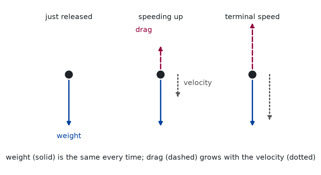
The weight does not change, but the drag follows the velocity, so the net force does not stay the same during a fall. The sketch shows three moments of one fall.

def draw_forces_on_a_falling_particle() -> Figure:
    """The forces on a falling particle at three moments, as a sketch."""
    weight_colour, drag_colour, velocity_colour = 0, 1, 2
    fig, ax = canvas(6.4, 3.8, (0, 10), (-0.1, 5.6))
    moments = (
        (1.8, "just released", 0.0),
        (5.0, "speeding up", 0.5),
        (8.2, "terminal speed", 1.0),
    )
    for x, moment, share in moments:
        circle(ax, (x, 3.2), 0.12, colour=INK, filled=True)
        text(ax, (x, 5.2), moment)
        arrow(ax, (x, 3.0), (x, 1.4), colour=weight_colour)
        if share:
            arrow(
                ax, (x, 3.4), (x, 3.4 + 1.6 * share), colour=drag_colour, linestyle="--"
            )
            arrow(
                ax,
                (x + 0.6, 3.2),
                (x + 0.6, 3.2 - 1.6 * share),
                colour=velocity_colour,
                linestyle=":",
            )
    text(ax, (1.8, 1.05), "weight", colour=weight_colour)
    text(ax, (4.7, 4.75), "drag", colour=drag_colour, ha="right")
    text(ax, (5.8, 2.9), "velocity", colour=velocity_colour, ha="left")
    text(
        ax,
        (5.0, 0.3),
        "weight (solid) is the same every time; drag (dashed) grows with the"
        " velocity (dotted)",
    )
    return fig

src/pbc/mechanics/experiments/newtons_laws.py, lines 40 to 73, read from the repository when this page was built.

Figure 1: conceptual Forces on a falling particle. The weight stays the same; the drag grows with the velocity, so the net force shrinks to zero.

The arrow lengths are drawn by eye, not measured. At release the net force is the weight alone; when the drag arrow is as long as the weight arrow the net force is zero and the velocity stops changing: the terminal speed.

The exact solution for linear drag

Write $\tau = m/b$, which has the dimension of a time. The velocity equation is then

$$\frac{\mathrm{d}\mathbf{v}}{\mathrm{d}t} = \mathbf{g} - \frac{\mathbf{v}}{\tau},$$

a linear first-order equation with constant coefficients. It has one constant solution, $\mathbf{v}_T = \mathbf{g}\,\tau$, at which the drag balances the weight: the terminal velocity. To find every other solution, write $\mathbf{u} = \mathbf{v} - \mathbf{v}_T$, the distance from the terminal velocity. Since $\mathbf{v}_T$ is constant and $\mathbf{g} - \mathbf{v}_T/\tau = 0$,

$$\frac{\mathrm{d}\mathbf{u}}{\mathrm{d}t} = \mathbf{g} - \frac{\mathbf{v}_T + \mathbf{u}}{\tau} = -\frac{\mathbf{u}}{\tau}.$$

A quantity whose rate of change is proportional to itself, with a negative constant, decays exponentially: $\mathbf{u}(t) = \mathbf{u}(0)\,e^{-t/\tau}$, as differentiating confirms. Back in terms of $\mathbf{v}$,

$$\mathbf{v}(t) = \mathbf{v}_T + (\mathbf{v}_0 - \mathbf{v}_T)\,e^{-t/\tau}.$$

The time constant $\tau$ is the time in which the remaining difference to the terminal velocity shrinks by the factor $e$; after $3\tau$ a fraction 0.050 of it is left, after $5\tau$ a fraction 0.0067. Integrating once more, with $\int_0^t e^{-s/\tau}\,\mathrm{d}s = \tau\,(1 - e^{-t/\tau})$, gives the position,

$$\mathbf{x}(t) = \mathbf{x}_0 + \mathbf{v}_T\,t + (\mathbf{v}_0 - \mathbf{v}_T)\,\tau\,\bigl(1 - e^{-t/\tau}\bigr).$$

Because the equation is linear, the components do not interact: the same formula holds on a line and in a plane, with $\mathbf{g}$ pointing down and $\mathbf{v}_0$ pointing wherever the particle was thrown. That is the property the next lesson loses.

Go deeper: The Coefficient of Drag (Russell Herman, LibreTexts Mathematics, 3.5.7, on the Stokes drag coefficient and the Newtonian regime; derivation.)

Why the drag is linear in the speed at low Reynolds number and quadratic at high: the drag coefficient of a sphere is $24/\mathrm{Re}$ in creeping flow, at $\mathrm{Re} \ll 1$, and approximately constant in the Newtonian drag regime at larger Reynolds number, though not at every large one. The lesson uses only the resulting force laws.

What explicit Euler does to it

The update rule can be solved exactly too. Substituting the acceleration into the velocity update and subtracting $\mathbf{v}_T$ on both sides gives

$$\mathbf{v}_{n+1} - \mathbf{v}_T = \Bigl(1 - \frac{\Delta t}{\tau}\Bigr)\,(\mathbf{v}_n - \mathbf{v}_T), \qquad\text{so}\qquad \mathbf{v}_n = \mathbf{v}_T + (\mathbf{v}_0 - \mathbf{v}_T)\, \Bigl(1 - \frac{\Delta t}{\tau}\Bigr)^{n}.$$

The computed velocity approaches the terminal velocity geometrically, by the factor $1 - \Delta t/\tau$ per step, where the exact solution uses the factor $e^{-\Delta t/\tau} = 1 - \Delta t/\tau + \tfrac{1}{2}(\Delta t/\tau)^2 - \dots$ The two agree to first order in $\Delta t$: they differ by $\tfrac{1}{2}(\Delta t/\tau)^2$ per step, and over $t/\Delta t$ steps that accumulates into an error proportional to $\Delta t$, as for every first-order method.

The formula also says what happens when the step is large. For $\Delta t > \tau$ the factor is negative: the computed velocity jumps past the terminal velocity and back, alternating sides. For $\Delta t > 2\tau$ the factor is less than $-1$, and the alternation grows without bound. The exact solution does nothing of the kind, because $e^{-\Delta t/\tau}$ is positive and below one for every step. This is instability, and it is a property of the method and the step, not of the physics. Numerically verified (linear drag, explicit Euler): Explicit Euler on linear drag converges to the terminal velocity only for $\Delta t < 2\tau$, and alternates around it for $\Delta t > \tau$. The first exercise runs into it on purpose.

The program

The reusable code lives in two modules of the repository, pbc.mechanics.dynamics and pbc.mechanics.drag. The listings in this section are read from those files when the site is built.

The state carries vectors now. Lists and numbers are converted, so that State(t=0.0, x=0.0, v=0.0) describes a particle on a line and State(t=0.0, x=[0.0, 0.0], v=[12.0, 15.0]) one in a plane:

@dataclass(frozen=True)
class State:
    """The particle at one instant: the time and the vectors of position
    and velocity.

    ``x`` and ``v`` are arrays of the same length, one entry per dimension
    of the motion: one for a line, two for a plane. Lists and numbers are
    converted.
    """

    t: float  # time, s
    x: Vector  # position, m
    v: Vector  # velocity, m/s

    def __post_init__(self) -> None:
        x = np.array(self.x, dtype=np.float64, ndmin=1)
        v = np.array(self.v, dtype=np.float64, ndmin=1)
        if x.ndim != 1 or x.shape != v.shape:
            raise ValueError(
                "x and v must be vectors of the same length,"
                f" got shapes {x.shape} and {v.shape}"
            )
        object.__setattr__(self, "x", x)
        object.__setattr__(self, "v", v)

src/pbc/mechanics/dynamics.py, lines 30 to 53, read from the repository when this page was built.

A force model is any function that takes the time, the position, and the velocity and returns the force as a vector of the same shape. Newton’s second law is the function that turns a mass and any number of force models into the acceleration function that a stepper needs:

def newton(mass: float, *forces: Force) -> Acceleration:
    """Newton's second law for a particle of ``mass`` (kg) under ``forces``.

    Returns the acceleration function a(t, x, v) = (sum of the forces) / m.
    Each force is a function F(t, x, v) that returns a vector in N.
    """
    if mass <= 0:
        raise ValueError(f"mass must be positive, got {mass}")

    def acceleration(t: float, x: Vector, v: Vector) -> Vector:
        total = np.zeros_like(x)
        for force in forces:
            total = total + force(t, x, v)
        return total / mass

    return acceleration

src/pbc/mechanics/dynamics.py, lines 80 to 95, read from the repository when this page was built.

The two force models of this lesson:

def weight(mass: float, g: ArrayLike) -> Force:
    """The weight m g of a particle of ``mass`` (kg).

    ``g`` is the gravitational acceleration as a vector in m/s² with the
    same number of entries as the position: ``[-9.81]`` on a vertical line
    with up positive, ``[0.0, -9.81]`` in a vertical plane with y upward.
    """
    force = mass * np.array(g, dtype=np.float64, ndmin=1)

    def weight_force(t: float, x: Vector, v: Vector) -> Vector:
        return force

    return weight_force

src/pbc/mechanics/dynamics.py, lines 98 to 110, read from the repository when this page was built.

def linear_drag(b: float) -> Force:
    """The linear drag force -b v, with the drag constant ``b`` in kg/s.

    For a sphere of radius r in a fluid of viscosity eta, Stokes' law gives
    b = 6 pi eta r.
    """
    if b < 0:
        raise ValueError(f"the drag constant must not be negative, got {b}")

    def drag(t: float, x: Vector, v: Vector) -> Vector:
        return -b * v

    return drag

src/pbc/mechanics/drag.py, lines 23 to 35, read from the repository when this page was built.

The stepper has the signature step(state, acceleration, dt). This is the stepping interface of the course: a later lesson adds steppers with the same signature, and the simulation loop below accepts any of them through its step argument. Explicit Euler is the only one so far:

The table gives the inputs, the output, and their units; the listing shows only the update, and each marked line has a note below it:

Inputs and outputs of euler_step.

Name	Kind	Type	Unit
state	input	State	t in s, x in m, v in m/s
acceleration	input	Acceleration	m/s²
dt	input	float	s
return	output	State	t in s, x in m, v in m/s

    return State(
        t=state.t + dt,
        x=state.x + state.v * dt,
        v=state.v + acceleration(state.t, state.x, state.v) * dt,
    )

1. Line 126, t=state.t + dt,: Time advances by the step, in seconds.
2. Line 127, x=state.x + state.v * dt,: The old velocity moves the particle: the position changes at the rate it had at the start of the step.
3. Line 128, v=state.v + acceleration(state.t, state.x, state.v) * dt,: The acceleration at the old state changes the velocity. Both lines read the old state, so their order does not matter; a stepper that used the new velocity for the position would be a different method.

src/pbc/mechanics/dynamics.py, lines 125 to 129, read from the repository when this page was built.

def simulate(
    initial: State,
    acceleration: Acceleration,
    dt: float,
    n_steps: int,
    step: Stepper = euler_step,
    until: Callable[[State], bool] | None = None,
) -> Trajectory:
    """Take up to ``n_steps`` steps of length ``dt`` (s) from ``initial``.

    ``step`` is the stepper; explicit Euler unless another is given. The
    trajectory holds the initial state and the state after every step. With
    ``until``, the simulation stops early, after the first state for which
    ``until(state)`` is true; that state is the last one of the trajectory.
    """
    if dt <= 0:
        raise ValueError(f"dt must be positive, got {dt}")
    if n_steps < 0:
        raise ValueError(f"n_steps must not be negative, got {n_steps}")
    states = [initial]
    for _ in range(n_steps):
        states.append(step(states[-1], acceleration, dt))
        if until is not None and until(states[-1]):
            break
    return Trajectory.of(states)

src/pbc/mechanics/dynamics.py, lines 132 to 156, read from the repository when this page was built.

The loop can also stop early, when a condition on the state becomes true; the third worked example uses that to stop a throw at the ground, and the next lesson relies on it. The exact solution for the fall with linear drag is the reference to compare with:

def fall_with_linear_drag(
    initial: State, mass: float, b: float, g: ArrayLike, t: ArrayLike
) -> Trajectory:
    """The exact motion of a particle of ``mass`` (kg) under its weight and
    linear drag with the constant ``b`` (kg/s), evaluated at the times ``t``.

    ``g`` is the gravitational acceleration as a vector in m/s², like the
    position. With the time constant tau = m / b and the terminal velocity
    v_T = g tau, the velocity relaxes towards v_T and the position follows:

        v(t) = v_T + (v_0 - v_T) exp(-(t - t_0) / tau),
        x(t) = x_0 + v_T (t - t_0) + (v_0 - v_T) tau (1 - exp(-(t - t_0) / tau)).

    ``t`` is a scalar or an array; the arrays of the result have one row per
    time. ``b`` must be positive: without drag the motion is the one of
    ``pbc.mechanics.kinematics.constant_acceleration``.
    """
    if mass <= 0:
        raise ValueError(f"mass must be positive, got {mass}")
    if b <= 0:
        raise ValueError(f"the drag constant must be positive, got {b}")
    tau = mass / b
    terminal = np.array(g, dtype=np.float64, ndmin=1) * tau
    times = np.array(t, dtype=np.float64, ndmin=1)
    elapsed = (times - initial.t)[:, np.newaxis]
    decay = np.exp(-elapsed / tau)
    excess = initial.v - terminal
    return Trajectory(
        t=times,
        x=initial.x + terminal * elapsed + excess * tau * (1.0 - decay),
        v=terminal + excess * decay,
    )

src/pbc/mechanics/drag.py, lines 64 to 95, read from the repository when this page was built.

Worked examples

Falling with linear drag

A particle is released from rest and falls against linear drag. On a vertical line the position is one number; the cell takes it as the distance fallen, so that down is positive and $\mathbf{g}$ is the vector [g]. The mass and the drag constant set the time constant $\tau = m/b$, which the cell computes.

mass = 0.5  # kg
b = 0.25  # drag constant, kg/s
tau = mass / b  # time constant, s
terminal_speed = g * tau  # m/s
down = [g]  # the gravitational acceleration, on a line with down positive

rest = State(t=0.0, x=0.0, v=0.0)
falling = newton(mass, weight(mass, down), linear_drag(b))
dt = 0.1  # time step, s
n_steps = 100

src/pbc/mechanics/experiments/newtons_laws.py, lines 24 to 33, read from the repository when this page was built.

def falling_particle(experiment: Experiment) -> tuple[Trajectory, Trajectory]:
    """Simulate the particle released from rest and evaluate the exact
    solution at the same instants; record the table of every tenth step."""
    euler = simulate(rest, falling, dt, n_steps)
    exact = fall_with_linear_drag(rest, mass, b, down, euler.t)

    experiment.table(
        "falling-particle",
        [
            (euler.t[i], euler.v[i, 0], exact.v[i, 0], euler.x[i, 0], exact.x[i, 0])
            for i in range(0, n_steps + 1, 10)
        ],
        columns=[
            ("t", "s", ".1f"),
            ("v Euler", "m/s", ".3f"),
            ("v exact", "m/s", ".3f"),
            ("x Euler", "m", ".3f"),
            ("x exact", "m", ".3f"),
        ],
        caption="Velocity and distance fallen, simulated and exact, every tenth "
        "step; to three decimals.",
    )
    return euler, exact

src/pbc/mechanics/experiments/newtons_laws.py, lines 76 to 98, read from the repository when this page was built.

Velocity and distance fallen, simulated and exact, every tenth step; to three decimals.

t (s)	v Euler (m/s)	v exact (m/s)	x Euler (m)	x exact (m)
0.0	0.000	0.000	0.000	0.000
1.0	7.870	7.717	3.873	4.179
2.0	12.582	12.398	14.062	14.431
3.0	15.404	15.237	28.033	28.366
4.0	17.093	16.959	44.268	44.535
5.0	18.104	18.003	61.858	62.060
6.0	18.710	18.637	80.260	80.406
7.0	19.072	19.021	99.149	99.251
8.0	19.289	19.254	118.328	118.398
9.0	19.419	19.395	137.681	137.729
10.0	19.497	19.481	157.139	157.171

The time constant is $\tau$ = 2.0 s and the terminal speed 19.613 m/s. Both velocities rise towards it, and after five time constants the exact one is within 0.7 per cent of it. The simulated velocity runs ahead of the exact one. The derivation says why: after $n$ steps the computed difference to the terminal velocity is $(1 - \Delta t/\tau)^n$ times the initial one, and $1 - \Delta t/\tau$ = 0.95 is smaller than $e^{-\Delta t/\tau}$ = 0.9512, so the computed velocity loses its initial difference a little faster at every step. The cell checks the formula directly:

def formula_gap(euler: Trajectory) -> float:
    """The largest difference between the simulated velocity and the
    formula for explicit Euler's v_n, in m/s."""
    n = np.arange(n_steps + 1)
    predicted = terminal_speed * (1 - (1 - dt / tau) ** n)
    return np.max(np.abs(euler.v[:, 0] - predicted))

src/pbc/mechanics/experiments/newtons_laws.py, lines 101 to 106, read from the repository when this page was built.

The largest difference between the simulation and the formula for $v_n$ is 1.1e-14 m/s, which is round-off. The program does exactly what the analysis of the method says it does, which is a stronger statement than “the error is small”.

def draw_fall_with_linear_drag(euler: Trajectory) -> Figure:
    """The velocity of the falling particle, explicit Euler against exact."""
    fine = np.linspace(0.0, euler.t[-1], 201)

    fig, ax = plt.subplots(figsize=(6.4, 3.6))
    ax.axhline(terminal_speed, color="#555555", linestyle=":", label="terminal speed")
    ax.plot(
        fine,
        fall_with_linear_drag(rest, mass, b, down, fine).v[:, 0],
        color="#00429d",
        label="exact",
    )
    ax.plot(
        euler.t,
        euler.v[:, 0],
        color="#93003a",
        linestyle="--",
        marker="o",
        markersize=3,
        label=f"explicit Euler, time step {dt} s",
    )
    ax.set_xlabel("time (s)")
    ax.set_ylabel("velocity (m/s)")
    ax.legend()
    return fig

src/pbc/mechanics/experiments/newtons_laws.py, lines 109 to 133, read from the repository when this page was built.

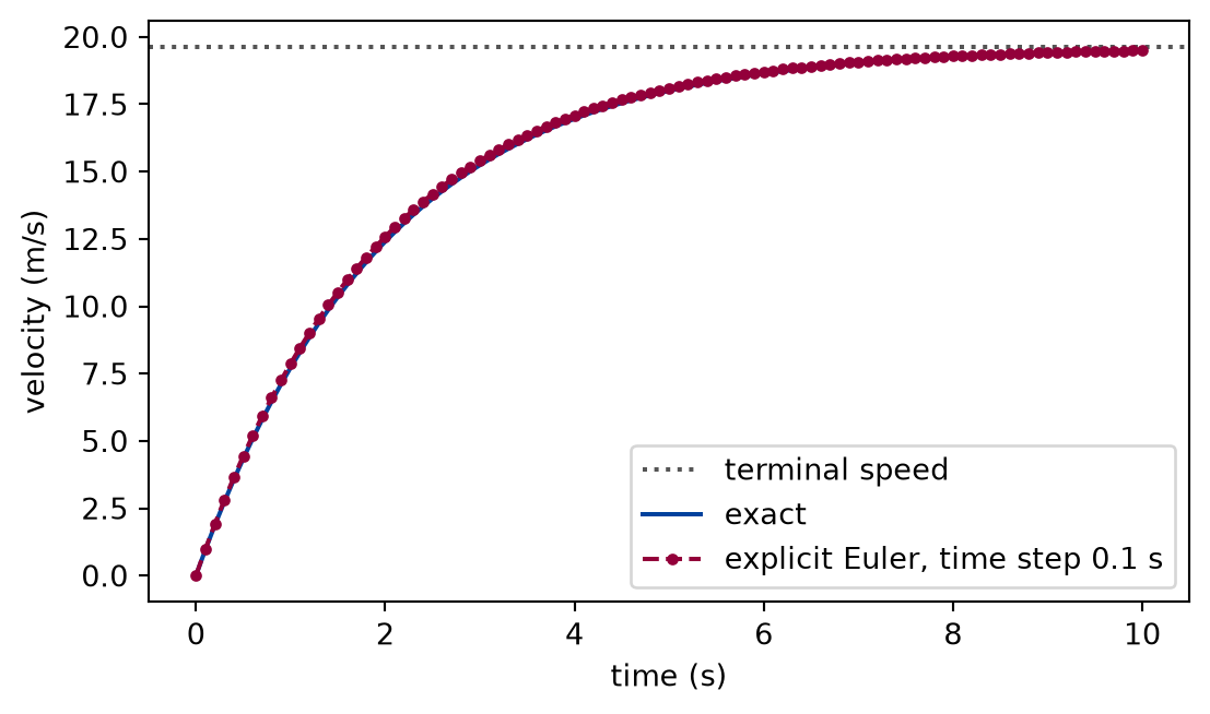
Figure 2: simulated Velocity of the falling particle: the coarse explicit Euler steps stay on the same side of the exact curve and close in on the terminal speed (dotted) a little faster than the exact solution does.

The figure shows what the formula predicted: the simulated curve never crosses the terminal speed, and the gap to the exact curve is the small difference between the factors $1 - \Delta t/\tau$ and $e^{-\Delta t/\tau}$, taken to the same power.

Halving the time step

The error after a fixed time should halve with the time step. The cell repeats the fall over the same duration with ever more steps and compares the velocity and the position at the end with the exact ones.

def final_errors(n):
    """Errors of the last simulated velocity and position, for n steps."""
    end = simulate(rest, falling, duration / n, n)
    reference = fall_with_linear_drag(rest, mass, b, down, end.t[-1])
    return end.v[-1, 0] - reference.v[0, 0], end.x[-1, 0] - reference.x[0, 0]

src/pbc/mechanics/experiments/newtons_laws.py, lines 136 to 140, read from the repository when this page was built.

def convergence(experiment: Experiment) -> np.ndarray:
    """The errors of the final velocity and position for each time step and
    the observed order of the position error; record their table."""
    errors = np.array([final_errors(n) for n in step_counts])
    orders = np.log2(errors[:-1, 1] / errors[1:, 1])

    experiment.table(
        "convergence",
        [
            (
                n,
                duration / n,
                errors[i, 0],
                errors[i, 1],
                orders[i - 1] if i else None,
            )
            for i, n in enumerate(step_counts)
        ],
        columns=[
            ("steps", "", "d"),
            ("time step", "s", ".6f"),
            ("v error", "m/s", ".6f"),
            ("x error", "m", ".6f"),
            ("observed order", "", ".3f"),
        ],
        caption="Error of the final velocity and position of the falling "
        "particle for each time step, and the observed order of the position "
        "error.",
    )
    return orders

src/pbc/mechanics/experiments/newtons_laws.py, lines 143 to 172, read from the repository when this page was built.

Error of the final velocity and position of the falling particle for each time step, and the observed order of the position error.

steps	time step (s)	v error (m/s)	x error (m)	observed order
100	0.100000	0.016032	-0.032065
200	0.050000	0.008138	-0.016277	0.978
400	0.025000	0.004100	-0.008199	0.989
800	0.012500	0.002057	-0.004115	0.995
1600	0.006250	0.001031	-0.002061	0.997
3200	0.003125	0.000516	-0.001032	0.999

Both errors halve with the step, and the observed order of the position error reaches 0.999 at the smallest step. Unlike the constant acceleration of the first lesson, where the ratio was exactly two, the order here approaches one gradually, because the dropped terms contain higher powers of $\Delta t / \tau$ as well.

A throw in the plane

The same functions run a motion in a plane; only the vectors have two components. The particle is thrown from the ground with a horizontal and an upward velocity, with $y$ upward so that $\mathbf{g}$ is [0, -g], and the loop stops at the first state below the ground. For comparison the cell also evaluates the drag-free motion, the parabola of the first lesson.

def on_the_ground(state):
    return state.x[1] < 0.0

src/pbc/mechanics/experiments/newtons_laws.py, lines 175 to 176, read from the repository when this page was built.

def throw():
    """A throw in the vertical plane with linear drag: the simulated flight,
    the exact one, the flight without drag, and the largest distance between
    the simulated and the exact position."""
    start = State(t=0.0, x=[0.0, 0.0], v=[12.0, 15.0])
    plane = [0.0, -g]
    thrown = newton(mass, weight(mass, plane), linear_drag(b))

    flight = simulate(start, thrown, 0.01, 10_000, until=on_the_ground)
    exact_flight = fall_with_linear_drag(start, mass, b, plane, flight.t)
    # The drag-free motion over its own, longer flight: back at the ground when
    # the vertical velocity has reversed, at t = 2 v_y / g.
    free_time = np.linspace(0.0, 2 * start.v[1] / g, 200)[:, None]
    without_drag = start.x + start.v * free_time + 0.5 * np.array(plane) * free_time**2

    largest_gap = np.max(np.linalg.norm(flight.x - exact_flight.x, axis=1))
    return flight, exact_flight, without_drag, largest_gap

src/pbc/mechanics/experiments/newtons_laws.py, lines 179 to 195, read from the repository when this page was built.

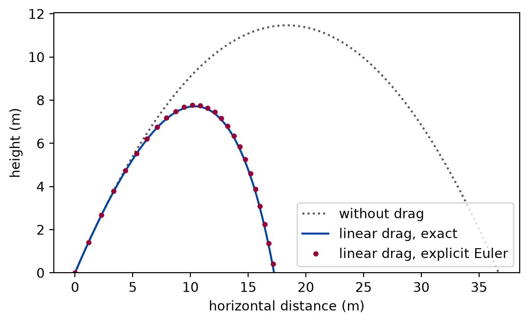
The particle is back at the ground after 2.55 s, 17.32 m away, and the largest distance between the simulated and the exact position along the way is 0.068 m.

def draw_throw_with_linear_drag(flight, exact_flight, without_drag) -> Figure:
    """The path of the throw with and without linear drag."""
    fig, ax = plt.subplots(figsize=(6.4, 3.6))
    ax.plot(
        without_drag[:, 0],
        without_drag[:, 1],
        color="#555555",
        linestyle=":",
        label="without drag",
    )
    ax.plot(
        exact_flight.x[:, 0],
        exact_flight.x[:, 1],
        color="#00429d",
        label="linear drag, exact",
    )
    ax.plot(
        flight.x[::10, 0],
        flight.x[::10, 1],
        color="#93003a",
        linestyle="none",
        marker="o",
        markersize=3,
        label="linear drag, explicit Euler",
    )
    ax.set_ylim(bottom=0.0)
    ax.set_xlabel("horizontal distance (m)")
    ax.set_ylabel("height (m)")
    ax.legend()
    return fig

src/pbc/mechanics/experiments/newtons_laws.py, lines 198 to 227, read from the repository when this page was built.

Figure 3: simulated Linear drag turns the symmetric parabola into a path that peaks earlier and falls more steeply; the explicit Euler points sit on the exact drag curve.

With drag the path is no longer a parabola: it rises less, peaks earlier, and comes down more steeply than it went up, because the drag takes away horizontal velocity all the time. Here the exact curve was still available to draw. For the quadratic drag of a ball in air there is none, and the next lesson shows how to trust a simulation without it.

Limits

• The exact solution exists only for linear drag and a constant force. The checks of this lesson compare a method with a solution; for the quadratic drag of the next lesson there is none.
• The stability result holds for explicit Euler on this one equation. It says nothing about the limits of other methods or of other forces, and the lesson does not measure them.
• Linear drag describes creeping flow only (fourth assumption); the examples use numbers chosen for readability, so no result here applies to a real falling object.
• The time step is never taken small enough to show round-off, and the second-order error terms are only argued, not isolated.
• The spring of the last exercise shows that explicit Euler misbehaves on an oscillation, but the lesson does not derive by how much; the next lesson does.

Self-check. A simulation of the falling particle with a time step of three time constants shows a velocity that jumps above and below the terminal speed and grows at every step. Does the real particle do that?

1. Yes. The drag and the weight compete, so the velocity can overshoot its limit.

   Not quite: the exact velocity approaches the terminal speed from one side and never crosses it, because the exponential factor is positive.

2. No. The oscillation belongs to the method: the factor $1 - \Delta t/\tau$ is below minus one for such a step, and the exact solution has no such factor.

   Correct: the sixth assumption fails, and the simulation reports its own time step, not the motion.

3. No. The oscillation is round-off, and a smaller number of digits would remove it.

   Not quite: the sequence follows from the update rule alone, in exact arithmetic too. Only a smaller time step removes it.

Solution to the self-check

For this step the computed difference to the terminal speed is multiplied by a factor below minus one at every step, so it alternates in sign and grows. The exact difference is multiplied by $e^{-\Delta t/\tau}$, which is between zero and one. The particle falls monotonically towards the terminal speed; the oscillating simulation is an artefact of a time step above twice the time constant.

Exercises

Exercise 1. Too large a step. The time constant of the falling particle is 2 s. Predict what explicit Euler computes for the velocity with a time step of 3 s and with one of 5 s, then run both for ten steps and look at the sequence of computed velocities.

Solution to exercise 1

The computed difference to the terminal velocity is multiplied by $1 - \Delta t/\tau$ at every step. With $\Delta t = 3$ s the factor is $-0.5$: the velocity jumps past the terminal speed, then back below it, with the overshoot halving every step. With $\Delta t = 5$ s the factor is $-1.5$: the same alternation, but growing by half every step, without bound.

def large_steps(experiment: Experiment) -> None:
    """Exercise 1: ten steps of 3 s and of 5 s; record their velocities."""
    runs = {step: simulate(rest, falling, step, 10) for step in (3.0, 5.0)}
    experiment.table(
        "large-step-velocity",
        [(i, runs[3.0].v[i, 0], runs[5.0].v[i, 0]) for i in range(11)],
        columns=[
            ("step", "", "d"),
            ("v, time step 3 s", "m/s", ".1f"),
            ("v, time step 5 s", "m/s", ".1f"),
        ],
        caption="Computed velocity of the falling particle for two large time steps.",
    )

src/pbc/mechanics/experiments/newtons_laws.py, lines 230 to 242, read from the repository when this page was built.

Computed velocity of the falling particle for two large time steps.

step	v, time step 3 s (m/s)	v, time step 5 s (m/s)
0	0.0	0.0
1	29.4	49.0
2	14.7	-24.5
3	22.1	85.8
4	18.4	-79.7
5	20.2	168.6
6	19.3	-203.8
7	19.8	354.7
8	19.5	-483.1
9	19.7	773.6
10	19.6	-1111.4

The first column settles at the terminal speed, the wrong way round but settling. The second leaves it further behind at every step. Nothing in the physics does this; the particle simply falls. The instability belongs to the method, and a simulation that shows it is reporting its own time step, not the motion.

Exercise 2. Time to terminal speed. How long does the particle released from rest take to reach 99 per cent of its terminal speed? Derive the answer from the exact solution, then find it from a simulation with a time step of 1 ms as the first instant at which the simulated speed exceeds that value.

Solution to exercise 2

From $v(t) = v_T\,(1 - e^{-t/\tau})$, the speed is $0.99\,v_T$ when $e^{-t/\tau} = 0.01$, that is at $t = \tau \ln 100$.

def time_to_terminal_speed():
    """Exercise 2: the time to 99 per cent of the terminal speed, exact and
    from a simulation with a step of 1 ms, in s."""
    predicted = tau * np.log(100)
    fine_fall = simulate(rest, falling, 0.001, 12_000)
    reached = fine_fall.t[np.argmax(fine_fall.v[:, 0] >= 0.99 * terminal_speed)]
    return predicted, reached

src/pbc/mechanics/experiments/newtons_laws.py, lines 245 to 251, read from the repository when this page was built.

The exact solution gives 9.210 s and the simulation 9.209 s. The simulation reaches the mark slightly early, as expected: the computed velocity runs ahead of the exact one. With a step of 1 ms the difference is of the order of the time step itself.

Exercise 3. A force that depends on position. Replace the drag by a spring that pulls the particle back to the origin with the force $F = -k\,x$, with $k = 2$ N/m, no gravity, and the particle released from rest at $x_0 = 1$ m. The exact motion is $x(t) = x_0 \cos(\omega t)$ with $\omega = \sqrt{k/m}$. Write the force model, simulate one full period with a time step of 10 ms, and compare the position at the end of the period with the exact one. What has happened to the amplitude?

Solution to exercise 3

The interface takes any function of time, position, and velocity, so the spring is one line. Nothing else changes.

k = 2.0  # spring constant, N/m
omega = np.sqrt(k / mass)
period = 2 * np.pi / omega

src/pbc/mechanics/experiments/newtons_laws.py, lines 256 to 258, read from the repository when this page was built.

def spring(t, x, v):
    return -k * x

src/pbc/mechanics/experiments/newtons_laws.py, lines 262 to 263, read from the repository when this page was built.

def one_period():
    """Exercise 3: one period of the spring with a time step of 10 ms."""
    released = State(t=0.0, x=1.0, v=0.0)
    return simulate(released, newton(mass, spring), 0.01, round(period / 0.01))

src/pbc/mechanics/experiments/newtons_laws.py, lines 266 to 269, read from the repository when this page was built.

The period is 3.142 s and the simulation ends at 3.14 s. The simulated position is then 1.0648 m, the exact one 1.0000 m, and the largest excursion so far is 1.0648 m.

The particle comes back further out than it started, and the excursion keeps growing in later periods. Explicit Euler uses the rates at the start of the step for the whole step, and on an oscillation that feeds energy in at every step; the harmonic oscillator lesson derives by how much. That lesson and the numerical integrators lesson introduce the steppers that avoid the growth. They plug into the same simulate through its step argument.

Run this experiment

This page was built from commit 6417e2ff90258bd2d2ba21d217eb7666fd24f680 of the repository.

In a clone at that commit, with the project’s Python packages installed, this command runs the experiment of this page:

uv run --locked --no-dev python -m pbc.mechanics.experiments.newtons_laws results

Files, tests, and every command

The files behind it:

• site/lessons/mechanics/02-newtons-laws/index.qmd: this page, with every code cell.
• src/pbc/mechanics/dynamics.py: code the experiment runs.
• src/pbc/mechanics/drag.py: code the experiment runs.
• src/pbc/mechanics/experiments/newtons_laws.py: code the experiment runs.
• src/pbc/experiment.py: code the experiment runs.
• tests/unit/test_dynamics.py: tests of that code.
• tests/unit/test_drag.py: tests of that code.
• tests/unit/test_newtons_laws_experiment.py: tests of that code.

With Git and uv installed (see the setup page), run:

git clone https://github.com/taspinar/physics-by-construction.git
cd physics-by-construction
git checkout 6417e2ff90258bd2d2ba21d217eb7666fd24f680
uv sync --locked --no-dev
uv run --locked --no-dev python -m pbc.mechanics.experiments.newtons_laws results

The experiment writes every figure of this page into results/, as <label>.png, and every number and table of the page, as the page shows it, into results/results.json. Its numbers match this page to the digits shown, and its figure files are the ones the page shows; digits beyond those can differ between machines, because floating-point libraries differ. Change the code of the experiment and run it again to see what changes.