Projectile motion with quadratic drag

A thrown ball with drag that grows with the square of its speed has no closed-form motion, so the simulation is validated by its limiting cases and by convergence, and then used to find the range against the launch angle.

Course

Classical mechanics, lesson 3 of 28

Slot

M3, Projectile motion with drag

Methods

Simulation

Difficulty

Intermediate, level 2 of 3

What you’ll learn

Validate a simulation without an exact solution by limiting cases and convergence
Read the order of convergence from a log-log plot
Find the launch angle of greatest range with and without drag

Prerequisites

Newton’s laws as a first-order system.

Before you begin

Trigonometry: the components of a vector at an angle
Logarithms: reading a log-log plot

Related

An agent runs an experiment

Previous

Newton’s laws as a first-order system

Next

The harmonic oscillator

With scripts, this page keeps a record in your browser of whether you completed the lesson. Nothing is stored without them.

With scripts, this place suggests what to do next, with the reason, from the progress saved in your browser. Without them, follow the learning path.

A ball thrown through air feels a drag that grows with the square of its speed and always points against its velocity. That couples the horizontal and the vertical motion: how fast the ball slows down horizontally depends on how fast it is falling, and the other way round. The equations of motion cannot be solved in closed form. Everything the previous lessons compared their simulations with is gone.

This lesson is about what to do then. The simulation is checked in the limiting cases that do have exact answers, without drag and in a long fall, and by refinement: a result that keeps changing as the time step shrinks is not a result yet, and the rate at which it stops changing says how far it is from the limit. With the simulation validated, the lesson uses it for a question that has no textbook answer: at what angle should the ball be thrown to go furthest? Without drag the answer is $45^\circ$ . With drag it is less, and by how much depends on the ball.

Assumptions

The model and the program rest on these assumptions. Each one names what goes wrong when it does not hold.

A point particle without spin. A spinning ball carries a layer of air around with it and feels a sideways force, the Magnus force, that makes topspin dip and backspin float. None of that is in the model; a real throw with spin lands somewhere else.
Quadratic drag with a constant drag coefficient. The drag is $-\tfrac{1}{2}\rho C_d A\,|\mathbf{v}|\,\mathbf{v}$ with a fixed $C_d$ . This holds in the Newtonian drag regime, where the drag coefficient of a sphere is approximately constant, so that the force scales with the speed squared, and the ball leaves a turbulent wake; the range is of the order of a thousand to a few hundred thousand (not verified), and the first example computes where the tennis ball lies in it. At much lower speeds the law becomes linear, as in the previous lesson. At higher speeds a smooth sphere reaches the drag crisis, where $C_d$ drops abruptly, by more than half (not verified); a rough or seamed ball reaches it earlier. For a ball thrown that fast the constant $C_d$ overestimates the drag. The lesson does not model either end of the range.
Still, uniform air. No wind, and a constant air density. In a wind the drag acts on the velocity relative to the air. Density changes with altitude by a few per cent per hundred metres, which matters for a shell, not for a ball.
Uniform gravity and flat ground at the launch height. The ranges are tens of metres, so the Earth’s curvature and rotation are negligible, and the ball lands at the height it was thrown from. A throw from a height is a one-argument change, shown in the code, but the formula for the drag-free range used as a check assumes a launch from the ground.
A first-order method with a small step. Explicit Euler’s error is proportional to the time step; the convergence study below measures it. The landing point is interpolated linearly within the last step, which adds an error proportional to the square of the step, below the method’s own. As in the previous lesson, a step that is too large makes the method unstable. Near a speed $v$ a small change $\delta v$ of the speed obeys $\mathrm{d}\,\delta v/\mathrm{d}t \approx -(2c\,v/m)\,\delta v$ , which is linear drag with the time constant $\tau = m/(2c\,v)$ , so the result of the previous lesson says the step must stay below $2\tau = m/(c\,v)$ . The first example puts a number on it, far above every step used.
Round-off is negligible. The steps are far above the resolution of double-precision numbers, so the errors in the tables are the errors of the method.

Drag that grows with the square of the speed

At everyday sizes and speeds a body moving through air leaves a turbulent wake, and the drag on it is

$\mathbf{F}_d = -c\,|\mathbf{v}|\,\mathbf{v}, \qquad c = \tfrac{1}{2}\,\rho\,C_d\,A,$

where $\rho$ is the density of the air, $A$ the cross-section the body presents to the flow, and $C_d$ a dimensionless drag coefficient that depends on the shape. The constant $c$ has the unit kg/m. The force has the magnitude $c\,|\mathbf{v}|^2$ and points against the velocity.

A body falling under this drag reaches the terminal speed at which the drag balances the weight, $c\,v_T^2 = m g$ , so

$v_T = \sqrt{\frac{m g}{c}}.$

Go deeper: The Coefficient of Drag (Russell Herman, LibreTexts Mathematics, 3.5.7, on the Stokes drag coefficient and the Newtonian regime; derivation.)

Why the drag is quadratic in the Newtonian drag regime, where the drag coefficient of a sphere is approximately constant, and linear at $\mathrm{Re} \ll 1$ . The lesson takes the quadratic law as its model and does not need the page.

The terminal speed is the natural scale of the problem. The ratio of the drag to the weight at any moment is $|\mathbf{v}|^2 / v_T^2$ . A ball thrown much more slowly than its terminal speed hardly notices the air; a ball thrown at its terminal speed starts with a drag equal to its weight, and its path looks nothing like a parabola.

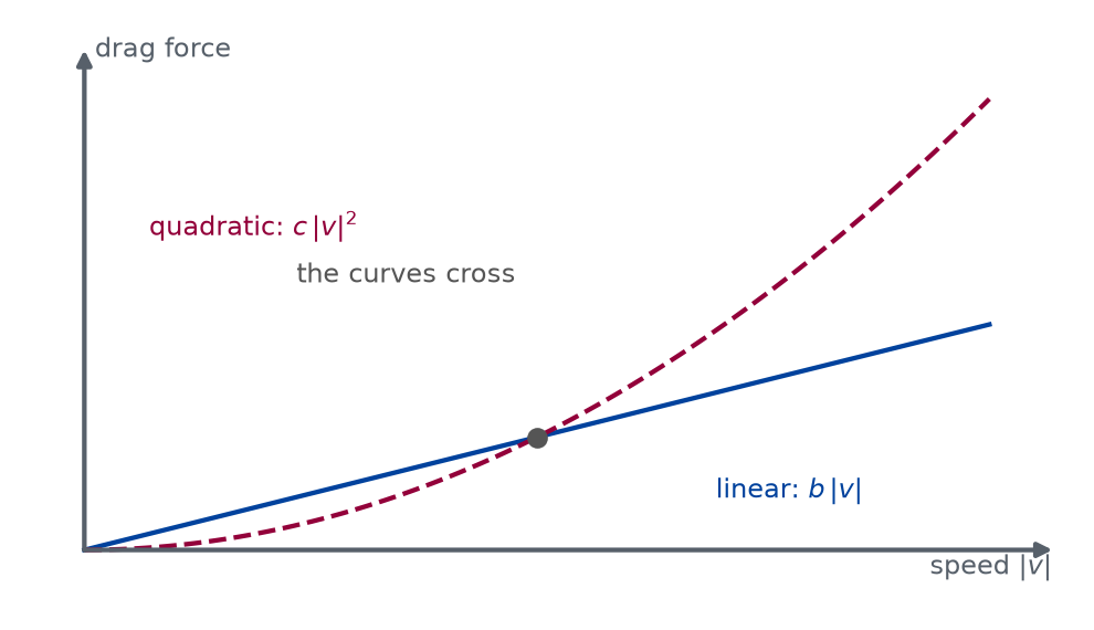
The two laws differ in how fast the drag grows with the speed.

def draw_drag_against_speed() -> Figure:
    """The linear and the quadratic drag law against speed, as a sketch."""
    fig, ax = canvas(6.4, 3.6, (0, 10), (0, 6))
    ax.set_aspect("auto")
    origin, width, height = 0.6, 8.6, 4.6
    arrow(ax, (origin, origin), (9.8, origin), colour=PAGE["muted"])
    arrow(ax, (origin, origin), (origin, 5.7), colour=PAGE["muted"])
    text(ax, (9.8, origin - 0.18), r"speed $|v|$", colour=PAGE["muted"], ha="right")
    text(ax, (origin + 0.1, 5.7), "drag force", colour=PAGE["muted"], ha="left")
    share = np.linspace(0.0, 1.0, 100)
    ax.plot(
        origin + width * share,
        origin + height * share / 2,
        color=FIGURE_COLOURS[0],
        linewidth=1.6,
    )
    ax.plot(
        origin + width * share,
        origin + height * share**2,
        color=FIGURE_COLOURS[1],
        linewidth=1.6,
        linestyle="--",
    )
    # The line height * share / 2 and the curve height * share**2 are equal at
    # share = 1/2, where both are height / 4: the marker is on both.
    ax.plot(
        [origin + width / 2], [origin + height / 4], marker="o", color=FIGURE_COLOURS[2]
    )
    text(ax, (6.6, 1.2), r"linear: $b\,|v|$", colour=0, ha="left")
    text(ax, (3.2, 3.9), r"quadratic: $c\,|v|^{2}$", colour=1, ha="right")
    text(ax, (4.7, 3.4), "the curves cross", colour=2, ha="right")
    return fig

src/pbc/mechanics/experiments/projectile_with_drag.py, lines 56 to 87, read from the repository when this page was built.

Sketch of drag force against speed. A solid line, the linear law, rises in a straight line from the origin. A dashed curve, the quadratic law, starts flatter and below the line, crosses it, and then climbs above it ever more steeply. — Figure 1: conceptual Drag against speed for the linear and the quadratic law. The quadratic drag is smaller at low speed and larger above the crossing.

The sketch has no scale, and where the curves cross depends on $b$ and $c$ . It carries the shape: doubling the speed doubles a linear drag and quadruples a quadratic one.

Why there is no closed form

With $x$ horizontal and $y$ upward, Newton’s second law reads

$\begin{aligned} m\,\frac{\mathrm{d}v_x}{\mathrm{d}t} &= -c\,\sqrt{v_x^2 + v_y^2}\;v_x, \\ m\,\frac{\mathrm{d}v_y}{\mathrm{d}t} &= -m g - c\,\sqrt{v_x^2 + v_y^2}\;v_y. \end{aligned}$

The square root contains both components, so neither equation can be solved on its own. For linear drag the factor in front of $v_x$ was the constant $b$ , the components separated, and each was a first-order linear equation with an exponential solution. Here the factor is the speed itself, which is unknown until the problem is solved. The motion can be reduced to integrals by a change of variables, but those integrals have to be evaluated numerically anyway, and there is no formula to compare a simulation with. This is an argument that the methods of the previous lessons do not apply, not a proof that no formula exists, and the lesson does not prove the latter.

How to trust a simulation without one

Three checks replace the comparison with an exact solution. Together they are the validation strategy of this lesson, and of every later one whose problem has no closed form.

Limiting cases. Set $c = 0$ and the motion must become the parabola of the first lesson, with the range $R_0 = v_0^2 \sin(2\theta) / g$ for a launch from the ground at speed $v_0$ and angle $\theta$ . The first lesson even predicts how far explicit Euler misses it: the computed height lags the exact one by $\tfrac{1}{2} g\,t\,\Delta t$ . At the landing time $T = 2 v_0 \sin\theta / g$ that lag is $v_0 \sin\theta\,\Delta t$ , and the ball is falling there with the vertical speed $v_0 \sin\theta$ , so it needs a time $\Delta t$ more to reach the ground: it lands $\Delta t$ late and so about $v_x \Delta t$ too far. A simulation that reproduces the parabola with exactly that error is doing what it should. The other limit, a long fall, must approach the terminal speed; the first exercise checks it.
Convergence. Compute the range with the step $\Delta t$ , then with $\Delta t/2$ , $\Delta t/4$ , and so on. For a first-order method the differences between successive results must halve each time, and the observed order, $\log_2$ of the ratio of successive differences, must tend to one. When it does, the result behaves like $R(\Delta t) = R^* + C\,\Delta t$ , and two steps determine both unknowns. Subtracting $R(\Delta t/2) = R^* + C\,\Delta t/2$ from $R(\Delta t)$ gives $C\,\Delta t/2 = R(\Delta t) - R(\Delta t/2)$ , and inserting it back gives $R^* \approx 2\,R(\Delta t/2) - R(\Delta t), \qquad R(\Delta t/2) - R^* \approx R(\Delta t) - R(\Delta t/2).$ This is Richardson extrapolation. The first formula estimates the limit, the second the error of the finer result, both from the simulation alone.
Physical sense. Drag must shorten the range, slow the ball down on the way up, and make the descent steeper than the ascent. These checks catch sign errors that the first two can miss.

Finding the ground

The simulation steps in time, and no step ends exactly at the ground. The loop stops after the first state below it, and the landing point is interpolated linearly between that state and the one before: if the last step went from a height $y_1 \ge 0$ to $y_2 < 0$ , the crossing happened a fraction $y_1 / (y_1 - y_2)$ of the way through the step, and the range is the horizontal position at that fraction. Within one step the path is nearly straight. Linear interpolation of a function $y(t)$ between two points $\Delta t$ apart has the error $\tfrac{1}{2}\,\ddot{y}(\xi)\,(t - t_1)(t - t_2)$ for some $\xi$ in the step, and $|(t - t_1)(t - t_2)|$ is largest at the middle of the step, where it is $\Delta t^2/4$ . So the interpolation is off by at most $\tfrac{1}{8}\,|\ddot{y}|\,\Delta t^2$ in height, far below the first-order error of the method itself.

The program

The code lives in the modules pbc.mechanics.drag and pbc.mechanics.projectile of the repository and runs on the stepping interface of the previous lesson. The listings in this section are read from those files when the site is built.

The force model and the constant it needs:

def quadratic_drag(c: float) -> Force:
    """The quadratic drag force -c |v| v, with the drag constant ``c`` in kg/m.

    ``c`` is 0 for no drag. For a body of cross-section area A in a fluid of
    density rho, c = rho C_d A / 2 with the dimensionless drag coefficient
    C_d of its shape; see ``drag_constant``.
    """
    if c < 0:
        raise ValueError(f"the drag constant must not be negative, got {c}")

    def drag(t: float, x: Vector, v: Vector) -> Vector:
        return -c * np.sqrt(v @ v) * v

    return drag

src/pbc/mechanics/drag.py, lines 38 to 51, read from the repository when this page was built.

def drag_constant(density: float, drag_coefficient: float, area: float) -> float:
    """The constant c = rho C_d A / 2 of quadratic drag, in kg/m.

    ``density`` is that of the fluid in kg/m³, ``drag_coefficient`` the
    dimensionless C_d of the body's shape, and ``area`` its cross-section
    facing the flow in m².
    """
    return 0.5 * density * drag_coefficient * area

src/pbc/mechanics/drag.py, lines 54 to 61, read from the repository when this page was built.

A throw starts from a speed, an angle, and a height:

def launch(speed: float, angle: float, height: float = 0.0) -> State:
    """The state at the moment of launch, at time 0.

    ``speed`` is in m/s, ``angle`` in degrees above the horizontal, and
    ``height`` the height above the ground in m.
    """
    if speed < 0:
        raise ValueError(f"speed must not be negative, got {speed}")
    radians = np.radians(angle)
    return State(
        t=0.0,
        x=[0.0, height],
        v=[speed * np.cos(radians), speed * np.sin(radians)],
    )

src/pbc/mechanics/projectile.py, lines 33 to 46, read from the repository when this page was built.

A flight is a simulation that stops at the ground, and the landing point is read off the last step:

def fly(
    initial: State,
    acceleration: Acceleration,
    dt: float,
    step: Stepper = euler_step,
    max_steps: int = 1_000_000,
) -> Trajectory:
    """Simulate from ``initial`` in steps of ``dt`` (s) until the particle has
    come down to the ground.

    The trajectory ends with the first state below the ground (y < 0), so
    that ``landing`` can interpolate the crossing. Raises ``RuntimeError``
    when the particle has not landed after ``max_steps`` steps.
    """

    def below_ground(state: State) -> bool:
        return state.x[1] < 0.0

    trajectory = simulate(initial, acceleration, dt, max_steps, step, below_ground)
    if trajectory.x[-1, 1] >= 0.0:
        raise RuntimeError(f"not landed after {max_steps} steps of {dt} s")
    return trajectory

src/pbc/mechanics/projectile.py, lines 49 to 70, read from the repository when this page was built.

def landing(trajectory: Trajectory) -> Landing:
    """The landing point of a flight, interpolated linearly between the last
    state above the ground and the first below it.

    ``trajectory`` is the result of ``fly``: its last state is the first one
    below the ground, and the state before it is on or above the ground.
    """
    y = trajectory.x[:, 1]
    if len(y) < 2 or y[-1] >= 0.0 or y[-2] < 0.0:
        raise ValueError(
            "the trajectory does not end with its first state below the ground;"
            " simulate the flight with fly()"
        )
    fraction = y[-2] / (y[-2] - y[-1])  # of the last step, until the crossing
    t = trajectory.t[-2] + fraction * (trajectory.t[-1] - trajectory.t[-2])
    x = trajectory.x[-2, 0] + fraction * (trajectory.x[-1, 0] - trajectory.x[-2, 0])
    return Landing(t=float(t), x=float(x))

src/pbc/mechanics/projectile.py, lines 81 to 97, read from the repository when this page was built.

The function that puts it all together answers the question of this lesson. It is the one an experiment, or an agent running an experiment, calls:

def projectile_range(
    speed: float,
    angle: float,
    mass: float,
    drag: float,
    dt: float,
    *,
    height: float = 0.0,
    g: float = STANDARD_GRAVITY,
    step: Stepper = euler_step,
) -> float:
    """The horizontal distance in m a projectile travels before it lands.

    The projectile of ``mass`` (kg) is launched at ``speed`` (m/s) and
    ``angle`` (degrees above the horizontal) from ``height`` (m) above flat
    ground, under gravity ``g`` (m/s², downward) and quadratic drag with the
    constant ``drag`` (kg/m; 0 for no drag). The flight is simulated in time
    steps of ``dt`` (s) with the stepper ``step``, explicit Euler by default,
    and the landing point is interpolated within the last step. The result
    depends on ``dt``: with explicit Euler its error is proportional to
    ``dt``, so halve ``dt`` until the digits you need stop changing.
    """
    acceleration = newton(mass, weight(mass, [0.0, -g]), quadratic_drag(drag))
    return landing(fly(launch(speed, angle, height), acceleration, dt, step)).x

src/pbc/mechanics/projectile.py, lines 100 to 123, read from the repository when this page was built.

The drag-free range for the first check:

def drag_free_range(speed: float, angle: float, g: float = STANDARD_GRAVITY) -> float:
    """The exact range in m without drag, for a launch from the ground:
    v² sin(2 theta) / g, with ``speed`` v in m/s, ``angle`` theta in degrees,
    and gravity ``g`` in m/s²."""
    return speed**2 * np.sin(np.radians(2.0 * angle)) / g

src/pbc/mechanics/projectile.py, lines 126 to 130, read from the repository when this page was built.

Worked examples

One throw

The ball is a tennis ball. Its mass and diameter are set in the cell; the density and viscosity of air at room temperature and the drag coefficient of a sphere in this range of speeds, about 0.5 (not verified), are inputs of the model, not results of it.

mass = 0.058  # kg
diameter = 0.067  # m
air_density = 1.2  # kg/m^3
air_viscosity = 1.8e-5  # Pa s
drag_coefficient = 0.5
c = drag_constant(air_density, drag_coefficient, np.pi * (diameter / 2) ** 2)
terminal_speed = np.sqrt(mass * g / c)

speed = 25.0  # launch speed, m/s
angle = 45.0  # launch angle, degrees
dt = 0.001  # time step, s
reynolds = air_density * speed * diameter / air_viscosity
stable_step = mass / (c * speed)  # largest stable step at the launch speed, s

src/pbc/mechanics/experiments/projectile_with_drag.py, lines 35 to 47, read from the repository when this page was built.

The drag constant is $c$ = 1.06e-03 kg/m and the terminal speed 23.2 m/s. The ball is thrown at about its terminal speed: the drag over the weight at launch is 1.16. The Reynolds number at launch is 1.1e+05, in the Newtonian drag regime, where a constant drag coefficient is a reasonable model, and the largest stable time step at the launch speed is 2.2 s, far above the time step 0.001 s used here.

The next cell simulates the throw with and without drag and tabulates what a thrower would want to know.

def throws(experiment: Experiment):
    """The same throw with and without quadratic drag; record their range,
    time of flight, and highest point."""
    down = [0.0, -g]
    ball_in_air = newton(mass, weight(mass, down), quadratic_drag(c))
    ball_in_vacuum = newton(mass, weight(mass, down))
    with_drag = fly(launch(speed, angle), ball_in_air, dt)
    without_drag = fly(launch(speed, angle), ball_in_vacuum, dt)

    experiment.table(
        "throws",
        [
            (name, landing(flight).x, landing(flight).t, flight.x[:, 1].max())
            for name, flight in (
                ("with drag", with_drag),
                ("without drag", without_drag),
            )
        ],
        columns=[
            ("throw", "", ""),
            ("range", "m", ".2f"),
            ("time of flight", "s", ".2f"),
            ("highest point", "m", ".2f"),
        ],
        caption="Range, time of flight, and highest point of the same throw "
        "with and without quadratic drag.",
    )
    return with_drag, without_drag

src/pbc/mechanics/experiments/projectile_with_drag.py, lines 90 to 117, read from the repository when this page was built.

Range, time of flight, and highest point of the same throw with and without quadratic drag.
throw	range (m)	time of flight (s)	highest point (m)
with drag	35.40	3.01	11.22
without drag	63.75	3.61	15.94

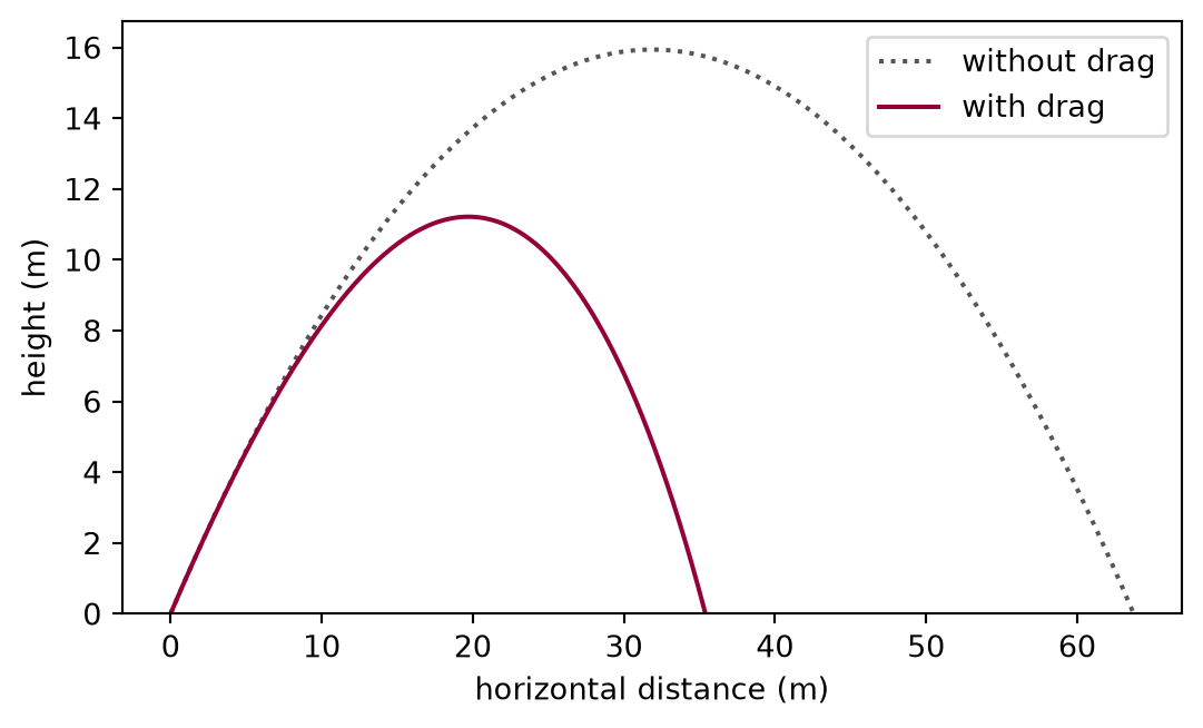
Drag takes away 44 per cent of the range. The exact drag-free range is 63.73 m, and the drag-free simulation is within 2 cm of it; the next example looks at that remaining difference. The paths show where the range goes:

def draw_throw_with_and_without_drag(with_drag, without_drag) -> Figure:
    """The paths of the throw with and without drag."""
    fig, ax = plt.subplots(figsize=(6.4, 3.6))
    ax.plot(
        without_drag.x[:, 0],
        without_drag.x[:, 1],
        color="#555555",
        linestyle=":",
        label="without drag",
    )
    ax.plot(with_drag.x[:, 0], with_drag.x[:, 1], color="#93003a", label="with drag")
    ax.set_ylim(bottom=0.0)
    ax.set_xlabel("horizontal distance (m)")
    ax.set_ylabel("height (m)")
    ax.legend()
    return fig

src/pbc/mechanics/experiments/projectile_with_drag.py, lines 120 to 135, read from the repository when this page was built.

Plot of height against horizontal distance in metres. The drag-free path is a symmetric parabola. The path with drag rises less high, peaks well before the midpoint of its flight, and comes down steeply to land little more than half as far. — Figure 2: simulated Drag removes the symmetry of the path: the ball with drag rises less, peaks early, and comes down steeply, because the drag has taken most of the horizontal velocity by then.

The path with drag is not a parabola. It comes down more steeply than it went up, because the drag has eaten most of the horizontal velocity by then, and it lands at a steeper angle and a lower speed than it was thrown with. The figure shows the shape of the path; the table above gives the numbers, which come from the same simulation.

The drag-free limit

The first check: with $c = 0$ the simulated range must approach the exact $R_0 = v_0^2 \sin(2\theta)/g$ as the step shrinks, and the first lesson predicts the error to be about $v_x\,\Delta t$ , the horizontal velocity times the time step.

def drag_free_convergence(experiment: Experiment):
    """The range of the drag-free throw for each time step against the exact
    range; record the table."""
    exact = drag_free_range(speed, angle)
    v_x = launch(speed, angle).v[0]
    steps = [0.1 / 2**k for k in range(8)]

    free_ranges = [projectile_range(speed, angle, mass, 0.0, step) for step in steps]

    experiment.table(
        "drag-free-convergence",
        [
            (step, computed, computed - exact, v_x * step)
            for step, computed in zip(steps, free_ranges, strict=True)
        ],
        columns=[
            ("time step", "s", ".6f"),
            ("range", "m", ".4f"),
            ("error", "m", ".4f"),
            ("v_x times time step", "m", ".4f"),
        ],
        caption="Range of the drag-free throw for each time step, its error "
        "against the exact range, and the error the first lesson predicts.",
    )
    return exact, v_x, steps, free_ranges

src/pbc/mechanics/experiments/projectile_with_drag.py, lines 138 to 162, read from the repository when this page was built.

Range of the drag-free throw for each time step, its error against the exact range, and the error the first lesson predicts.
time step (s)	range (m)	error (m)	v_x times time step (m)
0.100000	65.4977	1.7655	1.7678
0.050000	64.6150	0.8828	0.8839
0.025000	64.1737	0.4414	0.4419
0.012500	63.9530	0.2208	0.2210
0.006250	63.8427	0.1105	0.1105
0.003125	63.7875	0.0552	0.0552
0.001563	63.7599	0.0276	0.0276
0.000781	63.7461	0.0138	0.0138

The error halves with the step and matches the prediction from the first lesson to within the small interpolation error: at the smallest step the two differ by 6.2e-07 m. The simulation reproduces the one case that can be solved by hand, including the way it misses it.

Convergence with drag

The second check, on the throw with drag: the range at ever smaller steps, the difference to the previous one, the observed order, and the Richardson estimate of the limit from each pair of steps.

def richardson(experiment: Experiment, steps):
    """The range with drag for each time step, the observed order, and the
    Richardson estimate of the limit; record the table."""
    ranges = np.array([projectile_range(speed, angle, mass, c, step) for step in steps])
    differences = np.diff(ranges)
    orders = np.log2(differences[:-1] / differences[1:])
    limits = 2 * ranges[1:] - ranges[:-1]

    best_estimate = limits[-1]
    error_estimate = abs(differences[-1])

    experiment.table(
        "richardson",
        [
            (
                step,
                ranges[i],
                differences[i - 1] if i else None,
                orders[i - 2] if i >= 2 else None,
                limits[i - 1] if i else None,
            )
            for i, step in enumerate(steps)
        ],
        columns=[
            ("time step", "s", ".6f"),
            ("range", "m", ".4f"),
            ("difference", "m", ".4f"),
            ("observed order", "", ".3f"),
            ("estimated limit", "m", ".4f"),
        ],
        caption="Range with drag for each time step, the difference to the "
        "previous result, the observed order, and the Richardson estimate of "
        "the limit.",
    )
    return ranges, differences, orders, best_estimate, error_estimate

src/pbc/mechanics/experiments/projectile_with_drag.py, lines 165 to 199, read from the repository when this page was built.

Range with drag for each time step, the difference to the previous result, the observed order, and the Richardson estimate of the limit.
time step (s)	range (m)	difference (m)	observed order	estimated limit (m)
0.100000	35.8991
0.050000	35.6545	-0.2446		35.4099
0.025000	35.5278	-0.1267	0.949	35.4011
0.012500	35.4630	-0.0648	0.968	35.3982
0.006250	35.4306	-0.0324	0.998	35.3982
0.003125	35.4143	-0.0163	0.994	35.3980
0.001563	35.4061	-0.0082	0.996	35.3980
0.000781	35.4021	-0.0041	0.999	35.3980

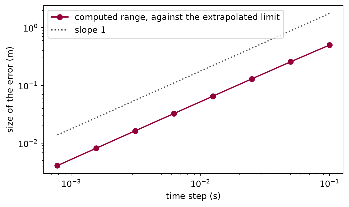
The differences halve and the observed order is 0.999 at the finest step, so the method behaves as a first-order method should on this problem too, and the Richardson estimates settle on a limit long before the direct results do. The range with drag is 35.398 m, and the finest direct result is still 4 mm from the previous one. The Richardson estimate assumes that the error is proportional to the time step; the observed orders are the check of that assumption, not a proof. On logarithmic axes the error of the direct results against the extrapolated limit is a straight line of slope one:

def draw_convergence_of_the_range(steps, ranges, best_estimate, v_x) -> Figure:
    """The error of the range with drag against the time step, log-log."""
    fig, ax = plt.subplots(figsize=(6.4, 3.6))
    ax.loglog(
        steps,
        np.abs(ranges - best_estimate),
        color="#93003a",
        marker="o",
        label="computed range, against the extrapolated limit",
    )
    ax.loglog(
        steps,
        np.array(steps) * v_x,
        color="#555555",
        linestyle=":",
        label="slope 1",
    )
    ax.set_xlabel("time step (s)")
    ax.set_ylabel("size of the error (m)")
    ax.legend()
    return fig

src/pbc/mechanics/experiments/projectile_with_drag.py, lines 202 to 222, read from the repository when this page was built.

Log-log plot of the error of the computed range in metres against the time step in seconds. The points lie on a straight line parallel to a dotted reference line of slope one: the error falls in proportion to the time step, over a wide span of both. — Figure 3: simulated The error of the range with drag falls in proportion to the time step, parallel to the reference line, so the extrapolated limit is a trustworthy reference.

The range against the launch angle

With the simulation validated and its error known, the question of the lesson. The cell computes the range for launch angles from $10^\circ$ to $80^\circ$ , with and without drag, using a step at which the convergence table puts the error well below a decimetre, and then finds the angle of the longest throw to a tenth of a degree with a one-dimensional minimiser from SciPy.

scan_dt = 0.002  # s
angles = np.arange(10.0, 80.5, 2.5)

src/pbc/mechanics/experiments/projectile_with_drag.py, lines 51 to 52, read from the repository when this page was built.

def best_angle(drag, ball_mass=mass):
    """The launch angle of the longest throw, to a tenth of a degree."""
    result = minimize_scalar(
        lambda a: -projectile_range(speed, a, ball_mass, drag, scan_dt),
        bounds=(20.0, 60.0),
        method="bounded",
        options={"xatol": 0.05},
    )
    return result.x, -result.fun

src/pbc/mechanics/experiments/projectile_with_drag.py, lines 225 to 233, read from the repository when this page was built.

def longest_throws(experiment: Experiment):
    """The range for each launch angle and the longest throw with and
    without drag; record the table of the longest throws."""
    ranges_with_drag = np.array(
        [projectile_range(speed, a, mass, c, scan_dt) for a in angles]
    )
    ranges_without = np.array(
        [projectile_range(speed, a, mass, 0.0, scan_dt) for a in angles]
    )

    best_with, furthest_with = best_angle(c)
    best_without, furthest_without = best_angle(0.0)

    experiment.table(
        "longest-throws",
        [
            ("with drag", furthest_with, best_with),
            ("without drag", furthest_without, best_without),
        ],
        columns=[
            ("throw", "", ""),
            ("longest range", "m", ".2f"),
            ("best angle", "degrees", ".1f"),
        ],
        caption="Longest range and the launch angle that gives it, found by a "
        "one-dimensional minimiser.",
    )
    return ranges_with_drag, ranges_without, best_with, best_without

src/pbc/mechanics/experiments/projectile_with_drag.py, lines 236 to 263, read from the repository when this page was built.

Longest range and the launch angle that gives it, found by a one-dimensional minimiser.
throw	longest range (m)	best angle (degrees)
with drag	35.74	40.5
without drag	63.77	45.0

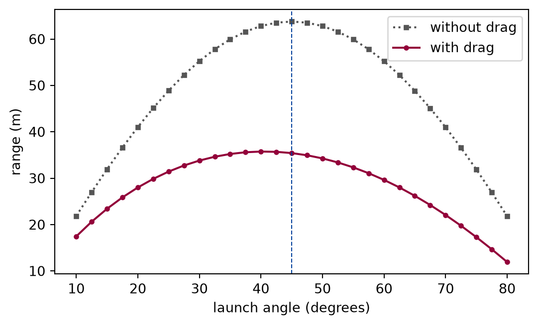
Without drag the longest throw is at $45^\circ$ , as the formula says, and the simulation finds it to the resolution asked of the minimiser: 45.0 degrees. With drag the best angle is 40.5 degrees, lower. Numerically verified (tennis ball at its launch speed): With quadratic drag the longest throw is flatter than $45^\circ$ for this ball. The lesson does not derive why. A steeper throw stays in the air longer and so spends more time losing speed to drag, which is the direction of the effect, but a flat throw also climbs less; the size of the shift comes from the simulation, not from this argument.

def draw_range_against_angle(ranges_with_drag, ranges_without) -> Figure:
    """The range against the launch angle, with and without drag."""
    fig, ax = plt.subplots(figsize=(6.4, 3.6))
    ax.plot(
        angles,
        ranges_without,
        color="#555555",
        linestyle=":",
        marker="s",
        markersize=3,
        label="without drag",
    )
    ax.plot(
        angles,
        ranges_with_drag,
        color="#93003a",
        marker="o",
        markersize=3,
        label="with drag",
    )
    ax.axvline(45.0, color="#00429d", linestyle="--", linewidth=0.8)
    ax.set_xlabel("launch angle (degrees)")
    ax.set_ylabel("range (m)")
    ax.legend()
    return fig

src/pbc/mechanics/experiments/projectile_with_drag.py, lines 266 to 290, read from the repository when this page was built.

Line plot of range in metres against launch angle in degrees. The drag-free curve is a symmetric arch peaking at a dashed vertical line at the forty-five degree mark. The curve with drag is much lower, peaks a few degrees to the left of the line, and is asymmetric: it falls off more steeply towards high angles than towards low ones. — Figure 4: simulated With drag the range is lower, its peak moves to a flatter angle, and the curve is lopsided: a throw that is too steep costs more than one that is too flat.

The curve with drag is not only lower but lopsided: it falls off more steeply towards high angles. How far the best angle moves below $45^\circ$ depends on the ratio of the launch speed to the terminal speed, as the third exercise shows.

Limits

The model has a constant drag coefficient, no spin, no wind, and flat ground at the launch height (assumptions one to four). The best angle and the range found here belong to this model of a tennis ball, not to a real throw; the lesson compares the simulation with no measurement.
The Reynolds-number ranges and the drag crisis are order-of-magnitude statements marked as not verified in the lesson, and the one source of the register supports only the form of the two force laws.
The convergence study shows that the error behaves like a first-order error for one throw. The Richardson estimate assumes this; other throws, such as a very steep one, are not checked.
Validation by limiting cases and refinement shows that the program solves its equations, not that the equations describe a ball. Only an experiment could show the second.

Self-check. The simulated range with drag changes by less than a millimetre when the time step is halved once more. Does that show that the range of a real tennis ball thrown like this is known to a millimetre?

Yes. The method has converged, so the range is correct to that precision.

Not quite: convergence shows that the program solves its equations to that precision. The equations have a constant drag coefficient and no spin or wind.
No. It shows that the numerical error of this model is below a millimetre; the model itself is not that accurate.

Correct: convergence measures the error of the method, and the assumptions of the model, such as a constant drag coefficient, are a different and larger source of error.
No. A first-order method cannot reach that precision.

Not quite: a first-order method reaches any precision at enough steps, at a cost that grows in proportion; the second exercise measures it.

Solution to the self-check

The refinement and the Richardson estimate bound the error between the simulation and the exact solution of the model’s equations. They say nothing about the difference between the model and the thrown ball: the drag coefficient is an input of about the right size, and the spin and the wind are absent. The real range is uncertain by far more than a millimetre.

Exercises

Exercise 1. The other limit. Drop the tennis ball from rest from a great height and let it fall for 15 s. Check that its speed approaches the terminal speed derived above, and find the time at which it reaches 95 per cent of it. Use a time step of 1 ms.

Solution to exercise 1

On a vertical line with down positive the acceleration is $g - (c/m)\,v\,|v|$ , and the same functions run it with one-component vectors.

def terminal_fall():
    """Exercise 1: the ball dropped from rest, with quadratic drag; the
    speeds and the time it reaches 95 per cent of the terminal speed."""
    dropped = State(t=0.0, x=0.0, v=0.0)
    falling = newton(mass, weight(mass, [g]), quadratic_drag(c))
    fall = simulate(dropped, falling, 0.001, 15_000)
    speeds = fall.v[:, 0]
    reached = fall.t[np.argmax(speeds >= 0.95 * terminal_speed)]
    return fall, speeds, reached

src/pbc/mechanics/experiments/projectile_with_drag.py, lines 293 to 301, read from the repository when this page was built.

The terminal speed from the formula is 23.190 m/s; the speed after 15 s of falling is 23.189 m/s, and 95 per cent of the terminal speed is reached after 4.33 s. The speed creeps up to the terminal speed and stays below it, as it must: once the drag balances the weight there is no force left to accelerate the ball. The natural time scale is $v_T / g$ , the time gravity alone would need to produce the terminal speed; 95 per cent of it is reached after 1.8 of those.

Exercise 2. A step for a millimetre. From the convergence table, which time steps give a computed range with drag that is within 1 cm of the limit, without extrapolation? How small must the step be for 1 mm? Read the first answer from the Richardson error estimates in the table, and find the second by continuing the halving until the estimate drops below 1 mm.

Solution to exercise 2

The error estimate of each result is its difference to the previous one, and the estimates halve with the step, so every extra decimal digit costs a little more than three halvings.

def refine(experiment: Experiment, steps, differences, ranges):
    """Exercise 2: the time steps that bring the range within a centimetre,
    and further halvings until the estimated error is below a millimetre;
    record the table of the halvings."""
    within_a_centimetre = [
        step
        for step, error in zip(steps[1:], np.abs(differences), strict=True)
        if error < 0.01
    ]

    tolerance = 0.001  # m
    step = steps[-1]
    previous = ranges[-1]
    refinement = []
    while True:
        step /= 2
        current = projectile_range(speed, angle, mass, c, step)
        estimate = abs(current - previous)
        refinement.append((step, current, estimate))
        if estimate < tolerance:
            break
        previous = current

    experiment.table(
        "refinement",
        refinement,
        columns=[
            ("time step", "s", ".6f"),
            ("range", "m", ".4f"),
            ("estimated error", "m", ".5f"),
        ],
        caption="Further halvings of the time step until the estimated error "
        "is below the tolerance.",
    )
    return within_a_centimetre, step

src/pbc/mechanics/experiments/projectile_with_drag.py, lines 304 to 338, read from the repository when this page was built.

Further halvings of the time step until the estimated error is below the tolerance.
time step (s)	range (m)	estimated error (m)
0.000391	35.4000	0.00204
0.000195	35.3990	0.00102
0.000098	35.3985	0.00051

The steps of the table with an estimated error below one centimetre are the 2 finest, from 0.001563 s down. A millimetre needs a step of 0.10 ms, that is 30841 steps for one throw. That is still cheap here, but a first-order method pays for every extra digit with ten times the work. The integrators lesson introduces methods that get the same digit for a small fraction of the steps.

Exercise 3. A heavier ball. A steel ball of the same diameter as the tennis ball has a mass of about 1.23 kg, so the same drag constant and a terminal speed several times higher. Thrown at the same 25 m/s, by what fraction does drag shorten its range at 45 degrees, and where is its best angle? Compare with the tennis ball and explain the difference with the ratio of launch speed to terminal speed.

Solution to exercise 3

def steel_and_tennis(experiment: Experiment, best_with):
    """Exercise 3: a steel ball of the same size against the tennis ball;
    record the table."""
    steel_mass = 1.23  # kg
    steel_terminal_speed = np.sqrt(steel_mass * g / c)
    steel_range = projectile_range(speed, 45.0, steel_mass, c, scan_dt)
    steel_best, _ = best_angle(c, steel_mass)
    tennis_range = projectile_range(speed, 45.0, mass, c, scan_dt)
    free_range = projectile_range(speed, 45.0, mass, 0.0, scan_dt)

    experiment.table(
        "steel-and-tennis",
        [
            (
                "steel",
                steel_terminal_speed,
                (speed / steel_terminal_speed) ** 2,
                steel_range,
                100 * (1 - steel_range / free_range),
                steel_best,
            ),
            (
                "tennis",
                terminal_speed,
                (speed / terminal_speed) ** 2,
                tennis_range,
                100 * (1 - tennis_range / free_range),
                best_with,
            ),
        ],
        columns=[
            ("ball", "", ""),
            ("terminal speed", "m/s", ".1f"),
            ("drag over weight at launch", "", ".3f"),
            ("range at 45 degrees", "m", ".2f"),
            ("range lost to drag", "per cent", ".1f"),
            ("best angle", "degrees", ".1f"),
        ],
        caption="The steel ball and the tennis ball, launched at the same speed.",
    )
    return steel_terminal_speed, steel_range, tennis_range, free_range

src/pbc/mechanics/experiments/projectile_with_drag.py, lines 341 to 381, read from the repository when this page was built.

The steel ball and the tennis ball, launched at the same speed.
ball	terminal speed (m/s)	drag over weight at launch	range at 45 degrees (m)	range lost to drag (per cent)	best angle (degrees)
steel	106.8	0.055	61.16	4.1	44.7
tennis	23.2	1.162	35.41	44.5	40.5

For the steel ball the drag at launch is 5 per cent of the weight, so the path is nearly a parabola, the range is shortened by 4.1 per cent, and the best angle is just below $45^\circ$ . The tennis ball, thrown at its terminal speed, loses 44 per cent of its range, and its best angle moves several degrees down. The one number that matters is $(v_0 / v_T)^2$ , the drag over the weight at launch: it is set by the launch speed and the mass, size, and shape of the ball, and it is why a shot put is thrown as if there were no air while a shuttlecock is not.

Run this experiment

This page was built from commit 6417e2ff90258bd2d2ba21d217eb7666fd24f680 of the repository.

In a clone at that commit, with the project’s Python packages installed, this command runs the experiment of this page:

uv run --locked --no-dev python -m pbc.mechanics.experiments.projectile_with_drag results

Files, tests, and every command

The files behind it:

site/lessons/mechanics/03-projectile-motion-with-drag/index.qmd: this page, with every code cell.
src/pbc/mechanics/dynamics.py: code the experiment runs.
src/pbc/mechanics/drag.py: code the experiment runs.
src/pbc/mechanics/projectile.py: code the experiment runs.
src/pbc/mechanics/experiments/projectile_with_drag.py: code the experiment runs.
src/pbc/experiment.py: code the experiment runs.
tests/unit/test_dynamics.py: tests of that code.
tests/unit/test_drag.py: tests of that code.
tests/unit/test_projectile.py: tests of that code.
tests/unit/test_projectile_with_drag_experiment.py: tests of that code.

With Git and uv installed (see the setup page), run:

git clone https://github.com/taspinar/physics-by-construction.git
cd physics-by-construction
git checkout 6417e2ff90258bd2d2ba21d217eb7666fd24f680
uv sync --locked --no-dev
uv run --locked --no-dev python -m pbc.mechanics.experiments.projectile_with_drag results

The experiment writes every figure of this page into results/, as <label>.png, and every number and table of the page, as the page shows it, into results/results.json. Its numbers match this page to the digits shown, and its figure files are the ones the page shows; digits beyond those can differ between machines, because floating-point libraries differ. Change the code of the experiment and run it again to see what changes.