The harmonic oscillator

A mass on a spring as the test system of the course: its exact motion, its orbit in phase space, and the proof from the update rule that explicit Euler multiplies its energy by the same factor at every step.

Course

Classical mechanics, lesson 4 of 28

Slot

M4, Harmonic oscillator

Methods

Simulation

Difficulty

Intermediate, level 2 of 3

What you’ll learn

• Solve the mass on a spring exactly and draw its orbit in phase space
• Show from the update rule that explicit Euler multiplies the energy by a fixed factor each step
• Use the oscillator as the test system for a stepping method

Prerequisites

Newton’s laws as a first-order system.

Before you begin

• Calculus: the derivatives of sine and cosine, and checking a solution by substitution
• Logarithms: the natural logarithm and the exponential of a small number

Related

Proving what the simulation showed

Previous

Projectile motion with quadratic drag

Next

Numerical integrators

With scripts, this page keeps a record in your browser of whether you completed the lesson. Nothing is stored without them.

With scripts, this place suggests what to do next, with the reason, from the progress saved in your browser. Without them, follow the learning path.

The last exercise of the Newton’s laws lesson replaced the drag by a spring and found that the simulated particle came back further out than it started. This lesson is about that spring. A mass pulled back towards a rest position by a force proportional to its displacement is the harmonic oscillator, and it is the test system of the rest of the course: its exact motion is known for all time, and its energy is a quantity that must stay constant, which a simulation can be checked against at every single step.

The check fails for explicit Euler, and this time the failure can be computed exactly. From the update rule alone, one step multiplies the energy of the oscillator by $1 + \omega^2\,\Delta t^2$, whatever the state and however small the step. The lesson derives that factor, shows the program reproducing it to round-off, and measures what it costs to keep the growth small. The next lesson replaces the method; a later lesson in the formal proofs strand proves the identity.

Assumptions

The model and the program rest on these assumptions. Each one names what goes wrong when it does not hold.

1. Hooke’s law, $F = -k\,x$, for every displacement. The restoring force is proportional to the displacement from the rest position. Real springs obey it for small extensions and stiffen or yield beyond them, and a pendulum obeys it only for small angles. The results that depend on it, a period independent of the amplitude and an elliptical orbit in phase space, stop holding; the energy conservation lesson treats the pendulum at large amplitude.
2. No friction and no drag. The energy is conserved and the orbit closes. With drag the energy decays, and a method that feeds energy in can hide the decay: the second exercise constructs a simulation of a damped oscillator whose amplitude does not change.
3. A point particle on a massless spring, on a line. A spring with mass moves too and lowers the frequency; the correction for a uniform spring is about one third of its mass added to $m$ (not verified). The same code runs in a plane, with the spring equally stiff in every direction, as the third exercise shows.
4. Constant mass and spring constant. A spring that warms up or a load that changes needs a different model.
5. The time step is small compared with the period. The factor derived below holds for every step size; what the step size sets is how much energy is fed in per period. At $\omega\,\Delta t = 1$ the factor $1 + \omega^2\Delta t^2$ is two: the energy doubles at every step, which is $2\pi/(\omega\,\Delta t) \approx 6$ steps per period, and the simulation says nothing about the oscillator.
6. Round-off is negligible. The identity is checked below to the resolution of double-precision numbers, and the longest run on this page stays far above it, so that the deviations shown are round-off and the growth shown is the method.

A mass on a spring

A particle of mass $m$ on a spring with the spring constant $k$ feels the force $F = -k\,x$, so Newton’s second law reads

$$m\,\frac{\mathrm{d}^2 x}{\mathrm{d}t^2} = -k\,x, \qquad\text{or}\qquad \frac{\mathrm{d}^2 x}{\mathrm{d}t^2} = -\omega^2\,x \quad\text{with}\quad \omega = \sqrt{\frac{k}{m}}.$$

Sine and cosine are the functions whose second derivative is minus themselves, scaled, so

$$x(t) = x_0 \cos(\omega t) + \frac{v_0}{\omega}\,\sin(\omega t), \qquad v(t) = -x_0\,\omega\,\sin(\omega t) + v_0 \cos(\omega t)$$

solves the equation from any initial position $x_0$ and velocity $v_0$, as substitution confirms. The motion repeats after the period $T = 2\pi/\omega$. The period does not depend on the amplitude: a large swing and a small one take the same time, which is what makes a spring, or a pendulum at small angles, a clock. The angular frequency $\omega$ is the one scale of the problem; the only dimensionless measure of a time step is $\omega\,\Delta t$, the fraction of a radian the oscillation advances per step.

Phase space and energy

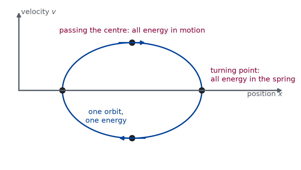
The state $(x, v)$ of the previous lessons can be drawn as a point in a plane with the position along one axis and the velocity along the other: the phase space of the oscillator. As time passes the point moves, and the exact motion traces a closed curve. Which curve follows from the energy,

$$E = \tfrac{1}{2}\,m\,v^2 + \tfrac{1}{2}\,k\,x^2,$$

the kinetic energy of the particle plus the energy stored in the spring. Its rate of change along the motion is

$$\frac{\mathrm{d}E}{\mathrm{d}t} = m\,v\,\frac{\mathrm{d}v}{\mathrm{d}t} + k\,x\,\frac{\mathrm{d}x}{\mathrm{d}t} = v\,(-k\,x) + k\,x\,v = 0.$$

The energy is conserved, so the point stays on the ellipse $\tfrac{1}{2} m v^2 + \tfrac{1}{2} k x^2 = E$, with the semi-axes $\sqrt{2E/k}$ along $x$ and $\sqrt{2E/m}$ along $v$, and goes round it once per period. Every state the simulation produces can be checked against this curve, not only against the exact position at one instant, and the check asks nothing of the method but one number per step. A simulation that leaves the ellipse has changed the energy, which the physics does not do.

def draw_oscillator_energy_ellipse() -> Figure:
    """The orbit of constant energy in phase space, as a sketch."""
    fig, ax = canvas(6.4, 4.4, (-5.8, 7.4), (-3.4, 3.9))
    arrow(ax, (-5.2, 0.0), (6.9, 0.0), colour=PAGE["muted"])
    arrow(ax, (-5.2, 0.0), (-5.2, 3.6), colour=PAGE["muted"])
    text(ax, (6.9, -0.18), "position $x$", colour=PAGE["muted"], ha="right")
    text(ax, (-5.1, 3.6), "velocity $v$", colour=PAGE["muted"], ha="left")
    ax.add_patch(
        Ellipse(
            (0, 0), 6.4, 4.4, fill=False, edgecolor=FIGURE_COLOURS[0], linewidth=1.6
        )
    )
    arrow(ax, (-0.6, 2.2), (0.6, 2.2), colour=FIGURE_COLOURS[0])
    arrow(ax, (0.6, -2.2), (-0.6, -2.2), colour=FIGURE_COLOURS[0])
    for point in ((3.2, 0.0), (0.0, 2.2), (-3.2, 0.0), (0.0, -2.2)):
        circle(ax, point, 0.12, colour=INK, filled=True)
    text(
        ax, (3.6, 0.7), "turning point:\nall energy in the spring", ha="left", colour=1
    )
    text(ax, (0.0, 2.75), "passing the centre: all energy in motion", colour=1)
    text(ax, (-1.2, -1.2), "one orbit,\none energy", colour=0)
    return fig

src/pbc/mechanics/experiments/harmonic_oscillator.py, lines 47 to 68, read from the repository when this page was built.

Figure 1: conceptual The exact motion in phase space is one ellipse of constant energy, traversed clockwise.

The ellipse is the curve $\tfrac{1}{2} m v^2 + \tfrac{1}{2} k x^2 = E$, drawn without a scale. At the ends of the position axis the energy sits in the spring; at the top and the bottom it is kinetic. The simulated orbits below are compared with this curve.

What explicit Euler does to it

The update rule of the previous lessons, with the acceleration $-\omega^2 x$, is

$$x_{n+1} = x_n + v_n\,\Delta t, \qquad v_{n+1} = v_n - \omega^2\,x_n\,\Delta t.$$

Take the energy after the step, in the form $E = \tfrac{1}{2} m\,(v^2 + \omega^2 x^2)$, and substitute:

$$\begin{aligned} v_{n+1}^2 + \omega^2 x_{n+1}^2 &= \bigl(v_n - \omega^2 x_n \Delta t\bigr)^2 + \omega^2 \bigl(x_n + v_n \Delta t\bigr)^2 \\ &= v_n^2 - 2\,\omega^2 x_n v_n \Delta t + \omega^4 x_n^2 \Delta t^2 + \omega^2 x_n^2 + 2\,\omega^2 x_n v_n \Delta t + \omega^2 v_n^2 \Delta t^2 \\ &= \bigl(v_n^2 + \omega^2 x_n^2\bigr)\bigl(1 + \omega^2 \Delta t^2\bigr). \end{aligned}$$

The cross terms cancel and what remains factorises. So

$$E_{n+1} = \bigl(1 + \omega^2\,\Delta t^2\bigr)\,E_n$$

at every step, for every state, and for every step size. The factor is never below one: explicit Euler feeds energy into the oscillator at each step, by an amount that does not depend on where in the oscillation the step is taken. After $n$ steps the energy is $(1 + \omega^2 \Delta t^2)^n E_0$ and the amplitude has grown by the square root of that. In phase space the computed point spirals outward, crossing ellipse after ellipse.

The same step has a geometric reading. Scale the velocity to $y = v/\omega$, so that the exact orbit is a circle, and write $h = \omega\,\Delta t$. The update rule then reads

$$\begin{pmatrix} x_{n+1} \\ y_{n+1} \end{pmatrix} = \begin{pmatrix} 1 & h \\ -h & 1 \end{pmatrix} \begin{pmatrix} x_n \\ y_n \end{pmatrix} = \sqrt{1 + h^2} \begin{pmatrix} \cos\varphi & \sin\varphi \\ -\sin\varphi & \cos\varphi \end{pmatrix} \begin{pmatrix} x_n \\ y_n \end{pmatrix}, \qquad \tan\varphi = h.$$

Each step is a stretch by $\sqrt{1 + h^2}$, whose square is the energy factor found above, and a rotation by the angle $\varphi = \arctan h$. The exact motion rotates by $h$ per step, and $\arctan h < h$ for $h > 0$, so the computed oscillation is slightly slow as well as growing.

Over a fixed time $t = n\,\Delta t$ the growth is $(1 + \omega^2 \Delta t^2)^{t/\Delta t}$, whose logarithm is $\tfrac{t}{\Delta t} \ln(1 + \omega^2 \Delta t^2) \approx \omega^2\,\Delta t\,t$ for small steps. The energy error after a fixed time is proportional to the step, as for every first-order method, and it never averages out: every step pushes the same way. Halving the step halves the logarithm of the growth, which is the convergence this lesson measures.

The program

The reusable code lives in the module pbc.mechanics.oscillator of the repository and runs on the stepping interface of the Newton’s laws lesson, with the same State, newton, and simulate. The listings in this section are read from the file when the site is built.

The force model is one line, and it serves on a line and in a plane:

def spring(k: float) -> Force:
    """Hooke's law: the force -k x towards the origin, with the spring
    constant ``k`` in N/m.

    The same function serves on a line and in a plane; in a plane it is an
    isotropic spring, equally stiff in every direction.
    """
    if k <= 0:
        raise ValueError(f"the spring constant must be positive, got {k}")

    def force(t: float, x: Vector, v: Vector) -> Vector:
        return -k * x

    return force

src/pbc/mechanics/oscillator.py, lines 20 to 33, read from the repository when this page was built.

The exact motion to compare with:

def angular_frequency(mass: float, k: float) -> float:
    """The angular frequency omega = sqrt(k / m) in rad/s of a particle of
    ``mass`` (kg) on a spring with the constant ``k`` (N/m). The period is
    2 pi / omega."""
    if mass <= 0:
        raise ValueError(f"mass must be positive, got {mass}")
    if k <= 0:
        raise ValueError(f"the spring constant must be positive, got {k}")
    return float(np.sqrt(k / mass))

src/pbc/mechanics/oscillator.py, lines 36 to 44, read from the repository when this page was built.

def harmonic_motion(initial: State, mass: float, k: float, t: ArrayLike) -> Trajectory:
    """The exact motion of a particle of ``mass`` (kg) on a spring with the
    constant ``k`` (N/m), evaluated at the times ``t``.

    With omega = sqrt(k / m) and the elapsed time s = t - t_0,

        x(t) = x_0 cos(omega s) + (v_0 / omega) sin(omega s),
        v(t) = -x_0 omega sin(omega s) + v_0 cos(omega s).

    The formula holds componentwise, so it serves on a line and in a plane.
    ``t`` is a scalar or an array; the arrays of the result have one row per
    time.
    """
    omega = angular_frequency(mass, k)
    times = np.array(t, dtype=np.float64, ndmin=1)
    phase = omega * (times - initial.t)[:, np.newaxis]
    cos, sin = np.cos(phase), np.sin(phase)
    return Trajectory(
        t=times,
        x=initial.x * cos + initial.v / omega * sin,
        v=-initial.x * omega * sin + initial.v * cos,
    )

src/pbc/mechanics/oscillator.py, lines 47 to 68, read from the repository when this page was built.

The energy of every state of a trajectory, the quantity the simulation is checked against:

def energy(trajectory: Trajectory, mass: float, k: float) -> NDArray[np.float64]:
    """The total mechanical energy in J at every instant of ``trajectory``:
    the kinetic energy m |v|² / 2 plus the potential energy k |x|² / 2 of
    the spring."""
    kinetic = 0.5 * mass * np.sum(trajectory.v**2, axis=1)
    potential = 0.5 * k * np.sum(trajectory.x**2, axis=1)
    return kinetic + potential

src/pbc/mechanics/oscillator.py, lines 71 to 77, read from the repository when this page was built.

The factor derived above, as a function so that the examples can compare the simulation with it:

def euler_energy_growth(mass: float, k: float, dt: float) -> float:
    """The factor 1 + omega² dt² = 1 + k dt² / m by which one explicit Euler
    step of length ``dt`` (s) multiplies the energy of the harmonic
    oscillator, whatever the state.

    The lesson derives it from the update rule; the formal proofs strand
    proves it. It is never less than 1: explicit Euler feeds energy into the
    oscillator at every step, by the same factor each time.
    """
    if dt <= 0:
        raise ValueError(f"dt must be positive, got {dt}")
    return 1.0 + angular_frequency(mass, k) ** 2 * dt**2

src/pbc/mechanics/oscillator.py, lines 80 to 91, read from the repository when this page was built.

Worked examples

Three periods

The oscillator of the examples is the one from the last exercise of the Newton’s laws lesson: half a kilogram on a spring of 2 N/m. It is pulled out to one metre and let go. The time step is a fraction of the period, which makes $\omega\,\Delta t$ the quantity to watch; the cell starts with 64 steps per period.

mass = 0.5  # kg
k = 2.0  # spring constant, N/m
omega = angular_frequency(mass, k)
period = 2 * np.pi / omega
released = State(t=0.0, x=1.0, v=0.0)  # pulled out 1 m and let go
oscillator = newton(mass, spring(k))

steps_per_period = 64
dt = period / steps_per_period
n_periods = 3

src/pbc/mechanics/experiments/harmonic_oscillator.py, lines 34 to 43, read from the repository when this page was built.

def three_periods(experiment: Experiment) -> tuple[Trajectory, Trajectory]:
    """Three periods with explicit Euler and the exact motion at the same
    instants; record the table of every half period."""
    euler = simulate(released, oscillator, dt, n_periods * steps_per_period)
    exact = harmonic_motion(released, mass, k, euler.t)

    experiment.table(
        "three-periods",
        [
            (
                euler.t[i],
                euler.x[i, 0],
                exact.x[i, 0],
                euler.v[i, 0],
                exact.v[i, 0],
            )
            for i in range(steps_per_period // 8, len(euler.t), steps_per_period // 2)
        ],
        columns=[
            ("t", "s", ".2f"),
            ("x Euler", "m", ".3f"),
            ("x exact", "m", ".3f"),
            ("v Euler", "m/s", ".3f"),
            ("v exact", "m/s", ".3f"),
        ],
        caption="Position and velocity of the mass on the spring, simulated and "
        "exact, every half period; to three decimals.",
    )
    return euler, exact

src/pbc/mechanics/experiments/harmonic_oscillator.py, lines 71 to 99, read from the repository when this page was built.

Position and velocity of the mass on the spring, simulated and exact, every half period; to three decimals.

t (s)	x Euler (m)	x exact (m)	v Euler (m/s)	v exact (m/s)
0.39	0.737	0.707	-1.466	-1.414
1.96	-0.867	-0.707	1.692	1.414
3.53	1.021	0.707	-1.952	-1.414
5.11	-1.202	-0.707	2.252	1.414
6.68	1.414	0.707	-2.597	-1.414
8.25	-1.664	-0.707	2.994	1.414

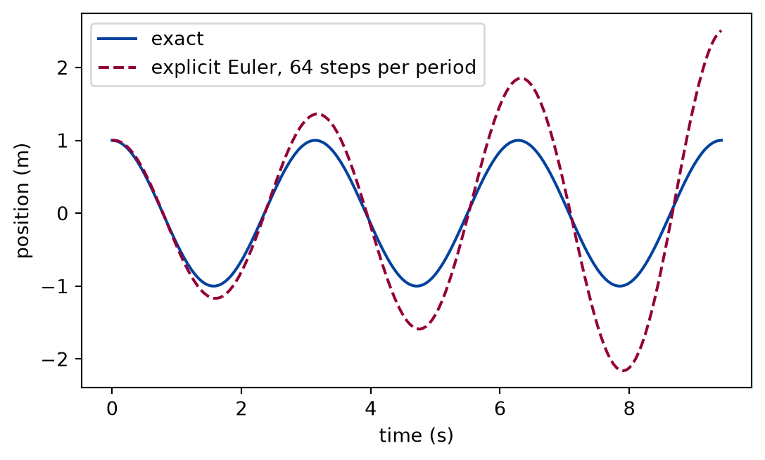
The angular frequency is $\omega$ = 2.0 rad/s, the period 3.1416 s, the time step 0.0491 s, and $\omega\,\Delta t$ = 0.0982. The rows are half a period apart, starting an eighth of a period in, so that neither column is at a zero crossing. The exact motion returns to the same two numbers every period. The simulated position swings further out at every turn, and the simulated velocity grows with it: in the third period the amplitude is 2.51 m instead of the one metre it started with.

def draw_oscillator_position(euler: Trajectory) -> Figure:
    """The position against time, explicit Euler against exact."""
    fine = np.linspace(0.0, euler.t[-1], 1001)

    fig, ax = plt.subplots(figsize=(6.4, 3.6))
    ax.plot(
        fine,
        harmonic_motion(released, mass, k, fine).x[:, 0],
        color="#00429d",
        label="exact",
    )
    ax.plot(
        euler.t,
        euler.x[:, 0],
        color="#93003a",
        linestyle="--",
        label=f"explicit Euler, {steps_per_period} steps per period",
    )
    ax.set_xlabel("time (s)")
    ax.set_ylabel("position (m)")
    ax.legend(loc="upper left")
    return fig

src/pbc/mechanics/experiments/harmonic_oscillator.py, lines 102 to 123, read from the repository when this page was built.

Figure 2: simulated The simulated oscillation grows at every swing while the exact one keeps its amplitude: explicit Euler adds energy at each step, and its peaks also fall a little late.

The orbit in phase space

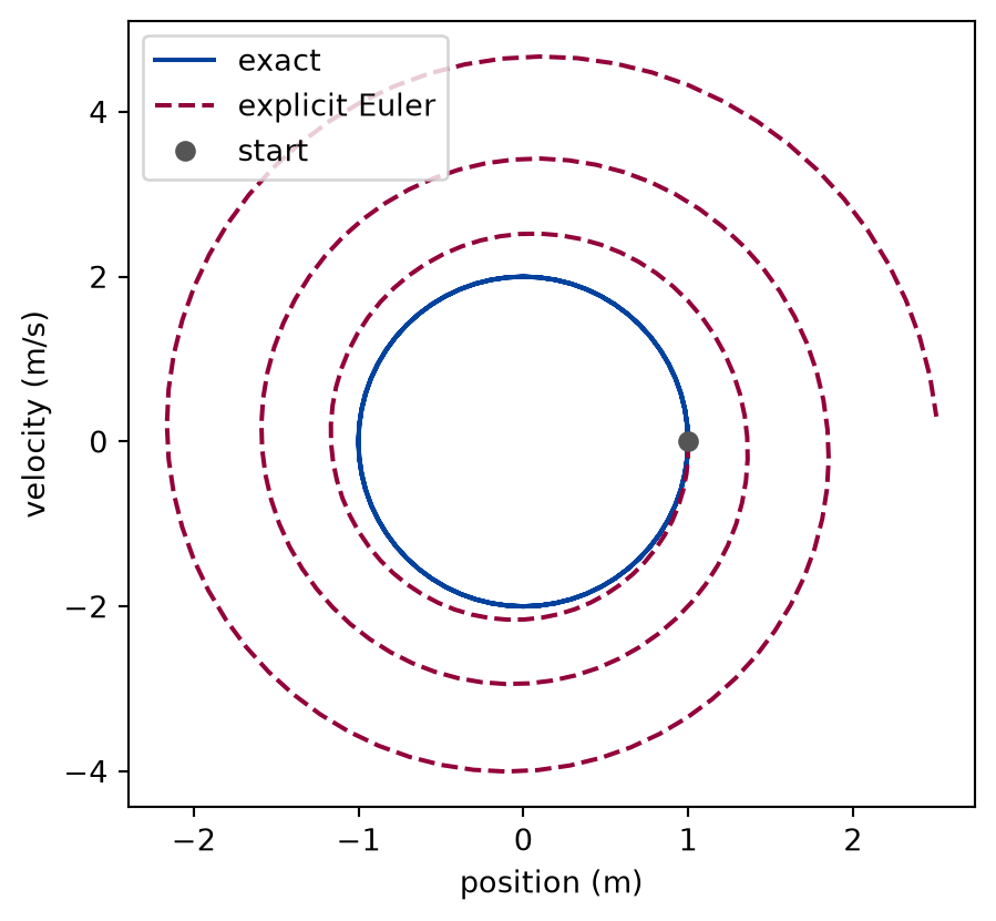
The same two trajectories, drawn as curves in the plane of position and velocity. The exact motion is the ellipse of constant energy; the simulation starts on it and spirals outward.

def draw_oscillator_phase_space(euler: Trajectory, exact: Trajectory) -> Figure:
    """The orbit in phase space, explicit Euler against exact."""
    fig, ax = plt.subplots(figsize=(6.4, 4.8))
    ax.plot(exact.x[:, 0], exact.v[:, 0], color="#00429d", label="exact")
    ax.plot(
        euler.x[:, 0],
        euler.v[:, 0],
        color="#93003a",
        linestyle="--",
        label="explicit Euler",
    )
    ax.plot(
        released.x[0],
        released.v[0],
        color="#555555",
        marker="o",
        linestyle="none",
        label="start",
    )
    ax.set_xlabel("position (m)")
    ax.set_ylabel("velocity (m/s)")
    ax.set_aspect(1 / omega)
    ax.legend(loc="upper left")
    return fig

src/pbc/mechanics/experiments/harmonic_oscillator.py, lines 126 to 149, read from the repository when this page was built.

Figure 3: simulated In phase space the exact orbit closes on the ellipse of constant energy, while explicit Euler never closes: it crosses to a larger ellipse at every turn.

The axes are scaled so that the exact orbit is a circle: along the vertical axis one unit of velocity is drawn as long as $1/\omega$ units of position. In these coordinates each step of explicit Euler is a turn by the angle $\arctan(\omega\,\Delta t)$ and a stretch by $\sqrt{1 + \omega^2 \Delta t^2}$, which is why the spiral looks the same from every direction. The figure shows the same data as the table, and the stretch is the energy factor derived above, to be checked next.

The energy, step by step

The derivation says that the energy after any step is the energy before it times $1 + \omega^2 \Delta t^2$. The cell computes the energy of every simulated state, divides each by the previous one, and compares all 192 ratios with the derived factor.

def energy_ratios(euler: Trajectory):
    """The energy at every step, the ratio of successive energies, the
    derived factor, and the largest deviation of a ratio from it."""
    energies = energy(euler, mass, k)
    ratios = energies[1:] / energies[:-1]
    factor = euler_energy_growth(mass, k, dt)

    deviation = np.max(np.abs(ratios - factor))
    return energies, ratios, factor, deviation

src/pbc/mechanics/experiments/harmonic_oscillator.py, lines 152 to 160, read from the repository when this page was built.

The energy at the start is 1.0000 J. The first six ratios of the energy after a step to the energy before it are 1.009638, 1.009638, 1.009638, 1.009638, 1.009638, 1.009638, and the derived factor $1 + \omega^2\Delta t^2$ is 1.009638. The largest deviation of any ratio from it is 4.4e-16. After 3 periods the energy is 6.307 times the initial energy, and the prediction is 6.307.

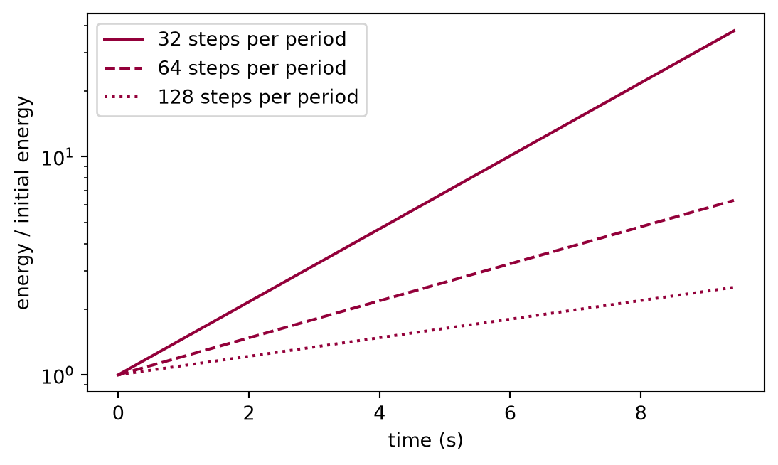
Numerically verified (explicit Euler on the harmonic oscillator, any step): Every ratio of successive energies equals the derived factor to round-off. This is a stronger statement than a small error. The program does exactly what the algebra says, including when the step is large, and the energy of the simulated oscillator can be written down for any step without running it. On a logarithmic axis the energy is a straight line whose slope is proportional to the step:

def draw_oscillator_energy_growth(initial_energy: float) -> Figure:
    """The energy over three periods for three time steps, on a log axis."""
    fig, ax = plt.subplots(figsize=(6.4, 3.6))
    for n, style in ((32, "-"), (64, "--"), (128, ":")):
        run = simulate(released, oscillator, period / n, n_periods * n)
        growth = energy(run, mass, k) / initial_energy
        ax.semilogy(
            run.t,
            growth,
            color="#93003a",
            linestyle=style,
            label=f"{n} steps per period",
        )
    ax.set_xlabel("time (s)")
    ax.set_ylabel("energy / initial energy")
    ax.legend(loc="upper left")
    return fig

src/pbc/mechanics/experiments/harmonic_oscillator.py, lines 163 to 179, read from the repository when this page was built.

Figure 4: simulated The energy grows as a straight line on a logarithmic axis, and the slope halves each time the step halves: the growth is a fixed factor per step.

Halving the time step

The logarithm of the growth over a fixed time is $\tfrac{t}{\Delta t}\ln(1 + \omega^2 \Delta t^2)$, which is proportional to $\Delta t$ for small steps. The cell doubles the number of steps per period and watches the logarithm of the energy growth after three periods halve.

def energy_growth(experiment: Experiment):
    """The energy growth over three periods for each time step and the
    observed order of its logarithm; record the table."""
    step_counts = [32 * 2**i for i in range(8)]
    growths = []
    for n in step_counts:
        run = simulate(released, oscillator, period / n, n_periods * n)
        end = energy(run, mass, k)
        growths.append(end[-1] / end[0])
    log_growths = np.log(growths)
    orders = np.log2(log_growths[:-1] / log_growths[1:])

    experiment.table(
        "energy-growth",
        [
            (
                n,
                2 * np.pi / n,
                growths[i],
                log_growths[i],
                orders[i - 1] if i else None,
            )
            for i, n in enumerate(step_counts)
        ],
        columns=[
            ("steps per period", "", "d"),
            ("omega dt", "", ".5f"),
            ("energy growth", "", ".4f"),
            ("ln(growth)", "", ".5f"),
            ("observed order", "", ".3f"),
        ],
        caption="Energy growth over three periods for each time step, its "
        "logarithm, and the observed order of that logarithm against the step.",
    )
    return step_counts, growths

src/pbc/mechanics/experiments/harmonic_oscillator.py, lines 182 to 216, read from the repository when this page was built.

Energy growth over three periods for each time step, its logarithm, and the observed order of that logarithm against the step.

steps per period	omega dt	energy growth	ln(growth)	observed order
32	0.19635	37.7709	3.63154
64	0.09817	6.3072	1.84169	0.980
128	0.04909	2.5198	0.92416	0.995
256	0.02454	1.5880	0.46250	0.999
512	0.01227	1.2602	0.23130	1.000
1024	0.00614	1.1226	0.11566	1.000
2048	0.00307	1.0595	0.05783	1.000
4096	0.00153	1.0293	0.02891	1.000

The observed order tends to one, from below: the logarithm of the factor is $\omega^2 \Delta t^2$ minus smaller terms, so coarse steps grow the energy a little less than the linear rule says. At 4096 steps per period the energy still grows by 2.9 per cent over three periods. The first exercise asks what one per cent costs.

Limits

• The energy factor is derived for explicit Euler on a linear spring. Other methods, and other forces, such as the pendulum at large amplitude, are not covered, and the numerical integrators lesson measures them one by one.
• The checks compare the simulation with the derived factor and with the exact motion. They do not show that a spring in a laboratory is a harmonic oscillator; that is the first assumption, and a measurement is needed to test it.
• The convergence table stops at a finite number of steps per period. The observed order tends to one in it, which is a measurement for these steps, not a proof for all steps.
• The exercise on damping shows that a wrong method can hide a physical effect; it does not say how to detect every such case.

Self-check. Explicit Euler multiplies the energy by $1 + \omega^2\Delta t^2$ at every step. With a fine time step the factor is very close to one. Is that enough to trust a long run?

1. Yes. A factor that close to one changes the energy by too little to matter.

   Not quite: the factors multiply. Over a fixed time the growth is proportional to the time step, and over a longer time it grows without bound.

2. No. The factor is the same at every step and never below one, so the small gains compound; a long enough run grows the energy by any amount.

   Correct: the logarithm of the growth is proportional to the time step and to the elapsed time, and nothing in the method pushes the energy back.

3. No. The growth averages out over a period, so only a short run is wrong.

   Not quite: every step pushes the same way, so there is nothing to average out.

Solution to the self-check

The growth over $n$ steps is $(1 + \omega^2\Delta t^2)^n$, the logarithm of which is about $\omega^2\,\Delta t\,t$ for a run of duration $t$. A finer step lowers the rate, not the sign: every step adds energy and none removes it. The run is trustworthy only for a duration short enough that this growth stays below the tolerance, which the first exercise computes.

Exercises

Exercise 1. The price of one per cent. How many steps per period does explicit Euler need for the energy of the oscillator to grow by at most one per cent over ten periods? Derive the answer from the factor, then confirm it with a simulation.

Solution to exercise 1

Ten periods take $n = 10 \cdot 2\pi / (\omega\,\Delta t)$ steps, so the growth is $(1 + \omega^2 \Delta t^2)^n$ with the logarithm $n \ln(1 + \omega^2 \Delta t^2) \approx 20\pi\,\omega\,\Delta t$. For a growth of at most $1.01$ that gives $\omega\,\Delta t \le \ln(1.01) / (20\pi)$, and the number of steps per period is $2\pi / (\omega\,\Delta t)$.

def one_per_cent():
    """Exercise 1: the steps per period that hold the energy within one per
    cent over ten periods, and the growth with them, in per cent."""
    largest_omega_dt = np.log(1.01) / (20 * np.pi)
    needed = int(np.ceil(2 * np.pi / largest_omega_dt))
    run = simulate(released, oscillator, period / needed, 10 * needed)
    end = energy(run, mass, k)
    growth_percent = 100 * (end[-1] / end[0] - 1)
    return needed, growth_percent

src/pbc/mechanics/experiments/harmonic_oscillator.py, lines 219 to 227, read from the repository when this page was built.

The simulation needs 39676 steps per period, and the energy after ten periods with them is 1.000 per cent above the start. That is 396760 steps in all to hold one per cent for ten periods. The next lesson holds the energy for a thousand periods with a few dozen steps per period, with a method that costs the same per step.

Exercise 2. A simulation that hides the damping. Add linear drag with the constant $b$ to the oscillator, so that the real motion loses energy and its amplitude decays. Explicit Euler feeds energy in at the rate $\omega^2 \Delta t$ per unit time, while the drag removes it at the rate $b/m$. Choose $b$ so that the two cancel, run five periods with 64 steps per period, and look at the amplitude. Then halve the step and look again.

Solution to exercise 2

The rates cancel when $b/m = \omega^2 \Delta t$, that is $b = k\,\Delta t$. The drag model of the Newton’s laws lesson plugs into newton next to the spring. The amplitude of each period is the largest distance from the rest position during it. For the real motion, with $\gamma = b/(2m)$ and $\omega_d = \sqrt{\omega^2 - \gamma^2}$, the exact solution from rest at one metre is

$$x(t) = e^{-\gamma t}\Bigl(\cos(\omega_d t) + \frac{\gamma}{\omega_d}\,\sin(\omega_d t)\Bigr),$$

as substitution into $m\ddot x = -k x - b \dot x$ confirms. Its velocity is $-(\omega_d + \gamma^2/\omega_d)\,e^{-\gamma t}\sin(\omega_d t)$, so the peaks fall at $t = n\pi/\omega_d$ and there $|x| = e^{-\gamma t}$ exactly: the curve $e^{-\gamma t}$ passes through the peaks, and over one undamped period $T$ it shrinks by the factor $e^{-bT/(2m)}$. The motion as a whole is bounded by the slightly larger envelope $\sqrt{1 + (\gamma/\omega_d)^2}\,e^{-\gamma t}$, which it touches just after each peak, where the cosine and sine terms combine. The damped oscillation is slightly slower than the undamped one, $\omega_d < \omega$, so each peak falls a little later than the start of its window of the undamped period, and the largest excursion in that window is $e^{-\gamma t}$ at the later peak time, a little below its value at the window boundary. The last column of the table is the largest excursion of this exact motion in each window of the undamped period, the same measure as the simulated columns, taken on a fine grid.

b = k * dt  # drag constant, kg/s
damped = newton(mass, spring(k), linear_drag(b))
gamma = b / (2 * mass)
omega_damped = np.sqrt(omega**2 - gamma**2)
decay = np.exp(-gamma * period)

src/pbc/mechanics/experiments/harmonic_oscillator.py, lines 232 to 236, read from the repository when this page was built.

def damped_motion(t):
    """The exact position of the damped oscillator released from 1 m."""
    damping = np.exp(-gamma * t)
    return damping * (
        np.cos(omega_damped * t) + gamma / omega_damped * np.sin(omega_damped * t)
    )

src/pbc/mechanics/experiments/harmonic_oscillator.py, lines 240 to 245, read from the repository when this page was built.

def largest_excursions(x, per_period):
    """The largest |x| in each of five periods, with that many samples per period."""
    return [
        np.max(np.abs(x[i * per_period : (i + 1) * per_period + 1])) for i in range(5)
    ]

src/pbc/mechanics/experiments/harmonic_oscillator.py, lines 248 to 252, read from the repository when this page was built.

def amplitudes(steps):
    """The largest excursion in each of five periods, with that many steps
    per period."""
    run = simulate(released, damped, period / steps, 5 * steps)
    return largest_excursions(run.x[:, 0], steps)

src/pbc/mechanics/experiments/harmonic_oscillator.py, lines 255 to 259, read from the repository when this page was built.

def damped_excursions(experiment: Experiment):
    """Exercise 2: the excursions of the simulated damped oscillator for three
    time steps and of the exact motion; record the table."""
    fine = np.linspace(0.0, 5 * period, 5 * 4096 + 1)
    real = largest_excursions(damped_motion(fine), 4096)

    simulated = [amplitudes(64), amplitudes(128), amplitudes(256)]

    experiment.table(
        "damped-excursions",
        [
            (i + 1, simulated[0][i], simulated[1][i], simulated[2][i], real[i])
            for i in range(5)
        ],
        columns=[
            ("period", "", "d"),
            ("64 steps", "m", ".3f"),
            ("128 steps", "m", ".3f"),
            ("256 steps", "m", ".3f"),
            ("real motion", "m", ".3f"),
        ],
        caption="Largest excursion in each of five periods of the simulated "
        "damped oscillator for three time steps, and of the exact motion.",
    )
    return simulated, real

src/pbc/mechanics/experiments/harmonic_oscillator.py, lines 262 to 286, read from the repository when this page was built.

Largest excursion in each of five periods of the simulated damped oscillator for three time steps, and of the exact motion.

period	64 steps (m)	128 steps (m)	256 steps (m)	real motion (m)
1	1.000	1.000	1.000	1.000
2	1.000	0.857	0.793	0.734
3	1.000	0.735	0.629	0.539
4	1.000	0.629	0.499	0.396
5	1.001	0.539	0.396	0.291

The drag constant is 0.0982 kg/s, and the peaks of the real motion shrink by the factor 0.735 per period.

With the coarsest step the simulated amplitude stays within 0.1 per cent of one metre for five periods, while the real amplitude falls to 0.29 m. Nothing in the output gives it away. Halving the step halves the artificial growth but not the drag, and the amplitude starts to decay; halving it again brings it closer to the real motion. A simulation of a damped oscillator whose amplitude does not change is reporting its time step, and the only way to catch it is to change the step and look again.

Exercise 3. In the plane. Let the spring pull towards the origin of a plane with the same stiffness in every direction, and start the mass at $(1, 0)$ m with the velocity $(0, 1)$ m/s. What orbit does the exact motion follow, and does the factor $1 + \omega^2 \Delta t^2$ still hold for the energy of each step?

Solution to exercise 3

The force $-k\,\mathbf{x}$ acts on each component separately, so each coordinate is a harmonic oscillator of its own with the same $\omega$: $x = \cos(\omega t)$ and $y = \tfrac{1}{\omega}\sin(\omega t)$, an ellipse with semi-axes $1$ m and $1/\omega$ m traced once per period. The algebra of the derivation used only that $\mathbf{x}\cdot\mathbf{v}$ cancels between the two cross terms, which holds for vectors too.

def in_a_plane(factor):
    """Exercise 3: an orbit in a plane; the exact orbit, the largest deviation
    of an energy ratio from ``factor``, and the largest distance from the
    exact position, in m."""
    in_plane = State(t=0.0, x=[1.0, 0.0], v=[0.0, 1.0])
    run = simulate(in_plane, oscillator, dt, 2 * steps_per_period)
    plane_exact = harmonic_motion(in_plane, mass, k, run.t)
    plane_energies = energy(run, mass, k)
    plane_ratios = plane_energies[1:] / plane_energies[:-1]

    plane_deviation = np.max(np.abs(plane_ratios - factor))
    plane_gap = np.max(np.linalg.norm(run.x - plane_exact.x, axis=1))
    return plane_exact, plane_deviation, plane_gap

src/pbc/mechanics/experiments/harmonic_oscillator.py, lines 289 to 301, read from the repository when this page was built.

The semi-axes of the exact orbit are 1.000 m and 0.500 m. The largest deviation of an energy ratio from the factor is 4.4e-16, and the largest distance between the simulated and the exact position over two periods is 0.847 m.

The factor holds to round-off in the plane as on the line. The energy growth of explicit Euler is a property of the method on this force, not of the dimension of the motion.

Run this experiment

This page was built from commit 6417e2ff90258bd2d2ba21d217eb7666fd24f680 of the repository.

In a clone at that commit, with the project’s Python packages installed, this command runs the experiment of this page:

uv run --locked --no-dev python -m pbc.mechanics.experiments.harmonic_oscillator results

Files, tests, and every command

The files behind it:

• site/lessons/mechanics/04-harmonic-oscillator/index.qmd: this page, with every code cell.
• src/pbc/mechanics/dynamics.py: code the experiment runs.
• src/pbc/mechanics/oscillator.py: code the experiment runs.
• src/pbc/mechanics/experiments/harmonic_oscillator.py: code the experiment runs.
• src/pbc/experiment.py: code the experiment runs.
• tests/unit/test_dynamics.py: tests of that code.
• tests/unit/test_oscillator.py: tests of that code.
• tests/unit/test_harmonic_oscillator_experiment.py: tests of that code.

With Git and uv installed (see the setup page), run:

git clone https://github.com/taspinar/physics-by-construction.git
cd physics-by-construction
git checkout 6417e2ff90258bd2d2ba21d217eb7666fd24f680
uv sync --locked --no-dev
uv run --locked --no-dev python -m pbc.mechanics.experiments.harmonic_oscillator results

The experiment writes every figure of this page into results/, as <label>.png, and every number and table of the page, as the page shows it, into results/results.json. Its numbers match this page to the digits shown, and its figure files are the ones the page shows; digits beyond those can differ between machines, because floating-point libraries differ. Change the code of the experiment and run it again to see what changes.