Energy conservation

Work, potential energy, and the pendulum at large amplitude, where no closed form gives the motion: the drift of the energy becomes the diagnostic of a simulation, with what it catches and what it does not.

Course

Classical mechanics, lesson 6 of 28

Slot

M6, Energy conservation

Methods

Simulation

Difficulty

Intermediate, level 2 of 3

What you’ll learn

• Compute work and potential energy along a simulated motion
• Simulate the pendulum at large amplitude
• Use the drift of the energy as a diagnostic, and say what it does not catch

Prerequisites

Numerical integrators.

Before you begin

• Calculus: the chain rule, the integral of a function along a path, and Taylor expansion to second order
• Trigonometry: the small-angle approximation of the sine
• Vectors: the dot product, and the gradient of a function of the position

Related

none

Previous

Numerical integrators

Next

Momentum and collisions

With scripts, this page keeps a record in your browser of whether you completed the lesson. Nothing is stored without them.

With scripts, this place suggests what to do next, with the reason, from the progress saved in your browser. Without them, follow the learning path.

A pendulum released from the side swings back and forth, and the first lesson of this course taught one way to check a simulation of such a motion: compare it with the exact solution. Every check so far did that: the parabola of the first lesson, the fall with linear drag, the cosine of the oscillator. Most forces have no such solution, and the pendulum is the simplest of them. Let the angle grow beyond a few degrees and the restoring force is no longer proportional to the displacement, the period depends on the amplitude, and no combination of elementary functions gives the angle as a function of time. A clock, a swing, and the escapement of a watch are pendulums of this kind. The question of the lesson is how to trust a simulation of a motion that nothing can be compared with.

What can be compared is the energy. For a force that depends on the position alone and does no net work around a closed path, the kinetic energy plus a potential energy is the same at every instant of the true motion. A simulation has no such law. Whether it keeps the energy, feeds it in, or drains it depends on the method and the step, as the previous lesson showed on the oscillator, where the exact result could be derived. This lesson turns that into a diagnostic: the drift of the energy over a run, one number computed from the trajectory alone, which shrinks at the order of the method and which catches a simulation that has changed the physics. The lesson also shows what the energy cannot see, because a diagnostic is only as good as its blind spots are known.

Assumptions

The model and the program rest on these assumptions. Each one names what goes wrong when it does not hold.

1. A rigid, massless rod of fixed length. The bob moves on a circle, so one coordinate describes it, and the tension in the rod does no work and is not modelled. A string goes slack above the horizontal when the bob is slow and the motion is no longer on the circle; a rod with mass changes the period.
2. No friction and no drag. The energy is conserved and the swing repeats forever. With drag the energy decreases, and the energy balance takes the place of its conservation: the second exercise checks that the loss equals the work done by the drag.
3. A conservative force. The potential energy exists because the tangential weight depends on the position alone and the work it does between two angles does not depend on the path. The energy diagnostic below needs such a force; for a force that depends on the velocity or on time there is no conserved energy to compare with.
4. Point mass, constant $g$ and $L$. The bob is a particle; a swinging body of finite size has a different period. The gravitational acceleration is uniform over the swing.
5. The step resolves the swing. The step is a fraction of the small-angle period. Near the top the bob moves slowly and the step is finer than it needs to be; through the bottom it moves fast, and the stated steps per period are chosen for there.
6. Round-off is negligible. The drifts reported below are far above the round-off of double precision; the Limits section puts the smallest of them next to it.

Work, energy, and the pendulum

A force $\mathbf F$ that acts on a particle moving with the velocity $\mathbf v$ does work at the rate $\mathbf F \cdot \mathbf v$. Newton’s second law and the chain rule turn that into a statement about the kinetic energy $K = \tfrac{1}{2} m |\mathbf v|^2$:

$$\frac{\mathrm{d}K}{\mathrm{d}t} = m\,\mathbf v \cdot \frac{\mathrm{d}\mathbf v}{\mathrm{d}t} = \mathbf v \cdot \mathbf F .$$

Integrated over a stretch of the motion, the change of kinetic energy equals the work $W = \int \mathbf F \cdot \mathrm{d}\mathbf x$ done by the force along the path: the work-energy theorem. It holds for every force, including drag.

A force that depends on the position alone is conservative when the work it does between two points is the same along every path. (On a region without holes, that is the same as saying that the force has no curl; the pendulum has one coordinate, where it holds trivially.) Then the work defines a function of the position, the potential energy $U(\mathbf x)$, through $W = -\Delta U$, and the force is minus its gradient, $\mathbf F = -\nabla U$. Along the motion $\mathrm{d}U/\mathrm{d}t = \nabla U \cdot \mathbf v = -\mathbf F \cdot \mathbf v = -\mathrm{d}K/\mathrm{d}t$, so

$$E = K + U \qquad\text{is constant.}$$

For the spring of the harmonic oscillator lesson, $U = \tfrac{1}{2} k x^2$ and this is the ellipse in phase space. The identity is all that the diagnostic needs: a trajectory whose energy changes has left the physics, and by how much the energy changed is a measure, in joules, of how far.

The pendulum on its arc

A bob of mass $m$ on a rod of length $L$ moves on a circle. Measure its position by the arc length $s = L\,\theta$ from the lowest point, with $\theta$ the angle of the rod from the vertical, so that the velocity along the arc is $v = L\,\dot\theta$ and the state $(s, v)$ is a position in metres and a velocity in metres per second, as in every lesson so far. The tension in the rod is perpendicular to the motion and does no work. The weight has the component $-m g \sin\theta$ along the arc, towards the bottom, so Newton’s second law along the arc is

$$m\,\frac{\mathrm{d}^2 s}{\mathrm{d}t^2} = -m\,g\,\sin\frac{s}{L}, \qquad\text{or}\qquad \ddot\theta = -\frac{g}{L}\,\sin\theta .$$

The potential energy follows from the height. At the angle $\theta$ the bob is $L(1 - \cos\theta)$ above the lowest point, and lifting the weight $m g$ through a height takes the work $m g$ times that height, so

$$U(s) = m\,g\,L\,\Bigl(1 - \cos\frac{s}{L}\Bigr), \qquad E = \tfrac{1}{2}\,m\,v^2 + m\,g\,L\,\Bigl(1 - \cos\frac{s}{L}\Bigr).$$

Differentiating confirms that this is the right potential: $-\mathrm{d}U/\mathrm{d}s = -m g \sin(s/L)$, the force above.

For small angles $\sin\theta \approx \theta$ and the force is $-(m g / L)\,s$: Hooke’s law with the spring constant $k = m g / L$, so the pendulum is the harmonic oscillator with $\omega_0 = \sqrt{g/L}$ and the small-angle period $T_0 = 2\pi\sqrt{L/g}$, independent of the amplitude. Beyond small angles the sine is smaller than its argument, the force is weaker than the linear one, and the bob takes longer to come back: the period grows with the amplitude.

The exact period and its series

For a release from rest at the angle $\theta_0$ the energy fixes the speed at every angle. Equating the energy at the angle $\theta$ with the energy at release, where $v = 0$, gives $\tfrac{1}{2} v^2 = g L (\cos\theta - \cos\theta_0)$, and with $v = L\dot\theta$ the angular velocity is $\dot\theta^2 = (2g/L)(\cos\theta - \cos\theta_0)$. The bob takes a quarter of the period to go from the release to the bottom, so

$$T = 4\int_0^{\theta_0} \frac{\mathrm{d}\theta}{\dot\theta} = 4\sqrt{\frac{L}{2g}}\int_0^{\theta_0} \frac{\mathrm{d}\theta}{\sqrt{\cos\theta - \cos\theta_0}} .$$

The integrand grows without bound at the release angle, but the integral converges. The substitution that tames it uses the identity $\cos\theta - \cos\theta_0 = 2\,(k^2 - \sin^2\tfrac{\theta}{2})$ with $k = \sin\tfrac{\theta_0}{2}$, and a new variable $\varphi$ defined by $\sin\tfrac{\theta}{2} = k \sin\varphi$, which runs from $0$ to $\pi/2$ while $\theta$ runs from $0$ to $\theta_0$. Then $\cos\theta - \cos\theta_0 = 2k^2\cos^2\varphi$ and $\mathrm{d}\theta = 2k\cos\varphi\,\mathrm{d}\varphi \big/ \sqrt{1 - k^2\sin^2\varphi}$, the factors $\cos\varphi$ cancel, and

$$T(\theta_0) = 4\sqrt{\frac{L}{g}}\;K(k^2), \qquad K(m) = \int_0^{\pi/2} \frac{\mathrm{d}\varphi}{\sqrt{1 - m\sin^2\varphi}}, \qquad k = \sin\frac{\theta_0}{2},$$

with $K$ the complete elliptic integral of the first kind, a function with no elementary form that SciPy evaluates. SciPy’s ellipk takes the parameter $m = k^2$, not the modulus $k$; other libraries and books use other conventions, so a value from one source cannot be compared with another without checking which. The integral diverges as $\theta_0$ approaches $\pi$, because $k$ approaches one and the integrand is then unbounded at the upper end: the bob lingers near the top.

For small amplitudes expand the integrand, $(1 - m\sin^2\varphi)^{-1/2} \approx 1 + \tfrac12 m\sin^2\varphi$. The integral of $\sin^2\varphi$ over the quarter circle is $\pi/4$, so

$$K(m) \approx \int_0^{\pi/2}\Bigl(1 + \tfrac12 m\sin^2\varphi\Bigr)\mathrm{d}\varphi = \frac{\pi}{2} + \frac{m}{2}\cdot\frac{\pi}{4} = \frac{\pi}{2}\Bigl(1 + \frac{m}{4}\Bigr).$$

Substituting into the period formula, with $T_0 = 2\pi\sqrt{L/g}$,

$$T \approx 4\sqrt{\frac{L}{g}}\,\frac{\pi}{2}\Bigl(1 + \frac{m}{4}\Bigr) = T_0\,\Bigl(1 + \frac{m}{4}\Bigr).$$

With $m = \sin^2(\theta_0/2) \approx \theta_0^2/4$ this is

$$T \approx T_0\,\Bigl(1 + \frac{\theta_0^2}{16}\Bigr),$$

which says that the period is longer than the small-angle period by one sixteenth of the squared amplitude in radians. The next term of the same expansion, with one more term of $K$ and of $\sin^2(\theta_0/2)$, is $11\,\theta_0^4/3072$. The first worked example compares both with the exact period.

Go deeper: Pendulum (mechanics) (Wikipedia contributors, Arbitrary-amplitude period, with "Power series solution for the elliptic integral"; derivation.)

The same integral, the same substitution, and the power series of the period to higher order, in one place, with a figure of how fast the truncated series approach the exact period. The lesson does not need it: the derivation above is complete.

Go deeper: scipy.special.ellipk (SciPy documentation, ellipk, definition and Notes on the parameterization; API documentation.)

The definition and the parameter convention of the function the program calls. It documents the function and derives nothing; it is the check that ellipk takes $k^2$.

What kind of motion the energy allows

The potential energy at the top is $2 m g L$. A pendulum with $E < 2 m g L$ cannot reach the top; it swings back and forth between the angles where $U = E$. One with $E > 2 m g L$ goes over the top and keeps rotating. The line $E = 2 m g L$ separates the two, and a pendulum on it needs an infinite time to arrive at the top, as the divergence of the period says. A simulation that lets the energy cross this line has not made a small error but changed the kind of motion.

Energy drift as a diagnostic

Let a simulation produce the states $(s_n, v_n)$ and compute the energy $E_n$ of each. The drift

$$\delta = \max_n \frac{|E_n - E_0|}{|E_0|}$$

is the largest fraction of the initial energy by which the run has strayed. It needs no exact solution, costs one evaluation of the potential per state, and needs $E_0 \neq 0$, which holds here because the bob is released from rest above the lowest point. The previous lesson derived what to expect of it on the oscillator, and this lesson measures it on the pendulum, where nothing is derived. For explicit Euler the runs below show it growing with the length of the run and never returning, and a later part derives why. For the symplectic methods, at a fixed step small enough for the method to be stable on the motion, the oscillator result is a band that does not grow; whether the pendulum behaves alike is a question for the measurement, and the lesson claims the band only for the runs it makes. The theory that predicts such a band for smooth potentials (backward error analysis) holds for times that are long but not infinite, and is outside this lesson.

If the drift of a method of order $p$ were governed by the error of the method, halving the step would divide it by $2^p$ or more. The drift of a sequence of runs with halving steps is therefore a convergence test that works without a formula for the motion, and the observed order is the logarithm to base two of the ratio of successive drifts. Whether the observed order equals the order of the method is something the table shows, not something the lesson assumes.

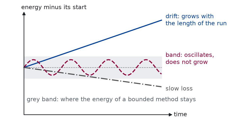
The three behaviours that the runs below measure can be told apart before any run, by what the energy does as the run gets longer:

def draw_energy_bands() -> Figure:
    """Drift, band, and slow loss of the energy, as a sketch."""
    t = np.linspace(0.0, 10.0, 400)
    fig, ax = diagrams.canvas(6.4, 3.2, (-1.4, 15.6), (-2.6, 2.8))
    ax.set_aspect("auto")
    ax.fill_between([0, 10], [-0.5, -0.5], [0.5, 0.5], color="#eaecf0", zorder=0)
    diagrams.arrow(ax, (0, -2.2), (0, 2.6), colour="#1f2328", width=1.0)
    diagrams.arrow(ax, (0, -2.2), (10.8, -2.2), colour="#1f2328", width=1.0)
    diagrams.line(ax, [(0, 0), (10, 0)], colour="#57606a", linestyle=":", width=1.0)
    diagrams.text(ax, (10.9, -2.2), "time", ha="left")
    diagrams.text(ax, (-0.2, 2.65), "energy minus its start", ha="left", va="bottom")
    ax.plot(t, 0.22 * t, color=FIGURE_COLOURS[0], linestyle="-", linewidth=1.6)
    ax.plot(
        t,
        0.36 * np.sin(2.3 * t),
        color=FIGURE_COLOURS[1],
        linestyle="--",
        linewidth=1.6,
    )
    ax.plot(t, -0.09 * t, color=FIGURE_COLOURS[2], linestyle="-.", linewidth=1.6)
    diagrams.text(
        ax, (10.3, 2.2), "drift: grows with\nthe length of the run", ha="left", colour=0
    )
    diagrams.text(
        ax, (10.3, 0.4), "band: oscillates,\ndoes not grow", ha="left", colour=1
    )
    diagrams.text(ax, (10.3, -1.0), "slow loss", ha="left", colour=2)
    diagrams.text(
        ax,
        (0.2, -1.5),
        "grey band: where the energy of a bounded method stays",
        ha="left",
        colour="#57606a",
    )
    return fig

src/pbc/mechanics/experiments/energy_conservation.py, lines 53 to 87, read from the repository when this page was built.

Figure 1: conceptual Three ways in which the energy of a simulation can stray, drawn as a sketch against the length of the run. Drift grows without limit, a band oscillates inside fixed bounds however long the run, and a slow loss falls steadily. Only a growth that never stops is a failure of the whole run; a band is a bounded error.

The sketch is not data; it fixes what the word “drift” will mean when the measured curves appear. A single drift number, the largest deviation, cannot tell a band from the beginning of a drift, which is why the runs below are made at several lengths.

What explicit Euler does to the energy

One step of explicit Euler moves the position with the old velocity, $s' = s + v\,\Delta t$, and the velocity with the old acceleration, $v' = v + a\,\Delta t$ with $a = F/m = -U'(s)/m$. The kinetic energy changes by $\tfrac12 m (v'^2 - v^2) = m v a\,\Delta t + \tfrac12 m a^2\Delta t^2$. The potential energy changes by

$$U(s + v\,\Delta t) - U(s) = U'\,v\,\Delta t + \tfrac12\,U''\,v^2\,\Delta t^2 + \dots,$$

and $U' = -m a$. The terms of first order in $\Delta t$ cancel, and what remains is

$$\Delta E \approx \tfrac12\,\Delta t^2\,\bigl(m a^2 + U''\,v^2\bigr).$$

For the oscillator, $U'' = k$ and the bracket is $2\omega^2 E$, the factor $1 + \omega^2\Delta t^2$ of the previous lesson, so the same formula covers both. For the pendulum, $U'' = (m g / L)\cos\theta$ is positive below the horizontal, so there both terms feed energy in: the first where the force is large, the second where the bob is fast. Above the horizontal $U''$ is negative and the second term takes energy out, but at rest the first term is positive in any case. The formula is a leading-order result in $\Delta t$ for one step; the worked example “One step of explicit Euler” checks it against the program.

What the drift cannot see

What the drift cannot see is a motion that stays on the right energy curve but moves along it at the wrong rate. A symplectic method with a bounded energy band has an error in the period of the order of the method, and over many periods the simulated bob falls steadily behind or ahead of the real one while its energy stays in the band. A phase error leaves the energy alone because the energy is the same at every point of the orbit. The worked example “What the energy does not see” measures that lag. The energy is a necessary check, not a sufficient one, and a run that passes it has passed one test.

The program

The reusable code lives in two modules of the repository, on the stepping interface of the earlier lessons. pbc.mechanics.energy has the energy of any trajectory under any potential, and the drift; pbc.mechanics.pendulum has the force and the potential of the pendulum and its periods. The listings in this section are read from the files when the site is built.

The energies take a potential as a function, so the same code serves every conservative force of the course. The drift is the one place where a choice of definition matters: it is measured against the size of the initial energy, so it is a fraction and has no unit.

def kinetic_energy(trajectory: Trajectory, mass: float) -> NDArray[np.float64]:
    """The kinetic energy m |v|² / 2 in J at every instant of ``trajectory``,
    for a particle of ``mass`` (kg)."""
    if mass <= 0:
        raise ValueError(f"mass must be positive, got {mass}")
    return 0.5 * mass * np.sum(trajectory.v**2, axis=1)

src/pbc/mechanics/energy.py, lines 29 to 34, read from the repository when this page was built.

def potential_energy(
    trajectory: Trajectory, potential: Potential
) -> NDArray[np.float64]:
    """The potential energy U(x) in J at every instant of ``trajectory``."""
    return np.array([potential(x) for x in trajectory.x], dtype=np.float64)

src/pbc/mechanics/energy.py, lines 37 to 41, read from the repository when this page was built.

def mechanical_energy(
    trajectory: Trajectory, mass: float, potential: Potential
) -> NDArray[np.float64]:
    """The mechanical energy, kinetic plus potential, in J at every instant
    of ``trajectory``: the quantity the true motion keeps constant."""
    return kinetic_energy(trajectory, mass) + potential_energy(trajectory, potential)

src/pbc/mechanics/energy.py, lines 44 to 49, read from the repository when this page was built.

def energy_drift(energies: NDArray[np.float64]) -> float:
    """The largest relative deviation of ``energies`` from the first one,
    max |E - E_0| / |E_0|: how far a simulation has let the energy go.

    The initial energy must not be zero; a bound orbit has a negative one,
    and the deviation is measured against its size.
    """
    initial = energies[0]
    if initial == 0:
        raise ValueError("the initial energy is zero; there is nothing to compare with")
    return float(np.max(np.abs(energies - initial)) / abs(initial))

1. Line 59, initial = energies[0]: The reference is the first energy of the run, not an exact value: the drift needs no solution of the motion.
2. Line 62, return float(np.max(np.abs(energies - initial)) / abs(initial)): The largest deviation over the whole run, in both directions, as a fraction of the size of the initial energy.

src/pbc/mechanics/energy.py, lines 52 to 62, read from the repository when this page was built.

The pendulum: the force along the arc as a force model for newton, its potential, and the two periods.

def pendulum_force(mass: float, length: float, g: float = STANDARD_GRAVITY) -> Force:
    """The force along the arc on a pendulum bob of ``mass`` (kg) on a rod
    of ``length`` (m): the tangential component -m g sin(s / L) of the
    weight, with the position s the arc length from the lowest point.

    For |s| much smaller than L it is -(m g / L) s, the spring of the
    harmonic oscillator lesson.
    """
    _check(mass, length, g)

    def force(t: float, x: Vector, v: Vector) -> Vector:
        return -mass * g * np.sin(x / length)

    return force

1. Line 47, return -mass * g * np.sin(x / length): The tangential component of the weight. The tension of the rod is absent because it is perpendicular to the motion.

src/pbc/mechanics/pendulum.py, lines 36 to 49, read from the repository when this page was built.

def pendulum_potential(
    mass: float, length: float, g: float = STANDARD_GRAVITY
) -> Potential:
    """The potential energy m g L (1 - cos(s / L)) in J of the bob at the arc
    length s: its weight times its height above the lowest point. It is 0 at
    the bottom and 2 m g L at the top, the energy that separates swinging
    from going over the top."""
    _check(mass, length, g)

    def potential(x: Vector) -> float:
        return float(mass * g * length * (1.0 - np.cos(x[0] / length)))

    return potential

1. Line 62, return float(mass * g * length * (1.0 - np.cos(x[0] / length))): The weight times the height of the bob above the lowest point. Its derivative with respect to the arc length is minus the force above.

src/pbc/mechanics/pendulum.py, lines 52 to 64, read from the repository when this page was built.

def small_angle_period(length: float, g: float = STANDARD_GRAVITY) -> float:
    """The period 2 pi sqrt(L / g) in s of a pendulum of ``length`` (m) at
    small amplitude, where it is a harmonic oscillator."""
    _check(None, length, g)
    return float(2.0 * np.pi * np.sqrt(length / g))

src/pbc/mechanics/pendulum.py, lines 67 to 71, read from the repository when this page was built.

def pendulum_period(
    length: float, amplitude: float, g: float = STANDARD_GRAVITY
) -> float:
    """The exact period in s of a pendulum of ``length`` (m) released from
    rest at the angle ``amplitude`` (rad), 0 <= amplitude < pi.

    With k = sin(amplitude / 2) the period is 4 sqrt(L / g) K(k²), where K
    is the complete elliptic integral of the first kind; it is the
    small-angle period at amplitude 0 and grows without bound as the
    amplitude approaches pi, the unstable rest position at the top.
    """
    _check(None, length, g)
    if not 0 <= amplitude < np.pi:
        raise ValueError(f"the amplitude must be in [0, pi), got {amplitude}")
    k = np.sin(0.5 * amplitude)
    return float(4.0 * np.sqrt(length / g) * ellipk(k**2))

1. Line 88, k = np.sin(0.5 * amplitude): The modulus of the elliptic integral, as in the derivation.
2. Line 89, return float(4.0 * np.sqrt(length / g) * ellipk(k**2)): SciPy takes the parameter, the square of the modulus, so the argument is the square of the sine.

src/pbc/mechanics/pendulum.py, lines 74 to 89, read from the repository when this page was built.

Worked examples

The period grows with the amplitude

The pendulum of the examples is one kilogram on a one-metre rod under the standard gravity. The cell releases it from rest at five amplitudes, runs three swings with the classical Runge-Kutta method at 200 steps per small-angle period, and measures the period from the times at which the bob passes the bottom moving forward, interpolated within the step. The exact period comes from the elliptic integral. The last two columns of the table are the series of the explanation, with one and with two terms.

mass = 1.0  # kg
length = 1.0  # m
pendulum = newton(mass, pendulum_force(mass, length))
potential = pendulum_potential(mass, length)
t0 = small_angle_period(length)
euler, symplectic_euler, verlet, rk4 = INTEGRATORS

src/pbc/mechanics/experiments/energy_conservation.py, lines 36 to 41, read from the repository when this page was built.

def released(degrees):
    """At rest at the given angle from the vertical."""
    return State(t=0.0, x=[length * np.radians(degrees)], v=[0.0])

src/pbc/mechanics/experiments/energy_conservation.py, lines 90 to 92, read from the repository when this page was built.

def run_swings(integrator, degrees, steps_per_period, n_swings):
    """n_swings of the pendulum released at the angle, with the small-angle
    period divided into steps_per_period steps."""
    swing = pendulum_period(length, np.radians(degrees))
    n_steps = round(n_swings * swing / t0 * steps_per_period)
    return simulate(
        released(degrees),
        pendulum,
        t0 / steps_per_period,
        n_steps,
        step=integrator.step,
    )

src/pbc/mechanics/experiments/energy_conservation.py, lines 95 to 106, read from the repository when this page was built.

def forward_crossings(trajectory):
    """The times at which the bob passes the bottom moving forward."""
    s, t = trajectory.x[:, 0], trajectory.t
    before = np.where((s[:-1] < 0) & (s[1:] >= 0))[0]
    fraction = -s[before] / (s[before + 1] - s[before])
    return t[before] + fraction * (t[before + 1] - t[before])

src/pbc/mechanics/experiments/energy_conservation.py, lines 109 to 114, read from the repository when this page was built.

def period_table(experiment: Experiment) -> list:
    """The period for five amplitudes from the elliptic integral, from a
    simulation, and from the series; record the table and return its rows."""
    rows = []
    for degrees in (10, 45, 90, 135, 170):
        angle = np.radians(degrees)
        exact = pendulum_period(length, angle)
        measured = np.mean(np.diff(forward_crossings(run_swings(rk4, degrees, 200, 3))))
        rows.append(
            (
                degrees,
                exact,
                exact / t0,
                measured,
                t0 * (1 + angle**2 / 16),
                t0 * (1 + angle**2 / 16 + 11 * angle**4 / 3072),
            )
        )

    experiment.table(
        "period-table",
        rows,
        columns=[
            ("amplitude", "degrees", "d"),
            ("exact period", "s", ".4f"),
            ("T / T0", "", ".4f"),
            ("simulated period", "s", ".4f"),
            ("one-term series", "s", ".4f"),
            ("two-term series", "s", ".4f"),
        ],
        caption="Period of the pendulum from the elliptic integral, from a "
        "simulation, and from the series, to four decimals.",
    )
    return rows

src/pbc/mechanics/experiments/energy_conservation.py, lines 117 to 150, read from the repository when this page was built.

Period of the pendulum from the elliptic integral, from a simulation, and from the series, to four decimals.

amplitude (degrees)	exact period (s)	T / T0	simulated period (s)	one-term series (s)	two-term series (s)
10	2.0102	1.0019	2.0102	2.0102	2.0102
45	2.0866	1.0400	2.0866	2.0838	2.0865
90	2.3682	1.1803	2.3682	2.3158	2.3596
135	3.0657	1.5279	3.0657	2.7026	2.9240
170	4.8944	2.4394	4.8944	3.1104	3.6672

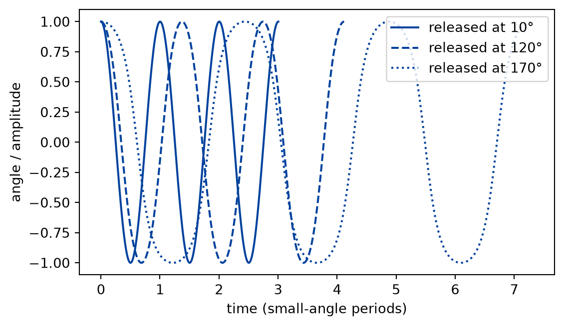
The small-angle period is 2.0064 s. Numerically verified (classical Runge-Kutta method, all five amplitudes of the table): The simulation reproduces the exact period to the four digits shown at every amplitude, so the force model and the period formula agree, and the amplitude dependence is real and large: at a right angle the period is 1.18 times the small-angle one, and near the top it is 2.4 times as long. The series is good where it is derived to be: at the smallest amplitude the one-term series is already within 6.7e-06 s of the exact period, the second term takes it to 1.3e-08 s, and at the largest amplitude both are far off, as an expansion in a small amplitude must be. The shape of the swing changes with the period:

def draw_pendulum_swings() -> Figure:
    """Three swings at three amplitudes, the angle over the amplitude."""
    fig, ax = plt.subplots(figsize=(6.4, 3.6))
    for degrees, style in ((10, "-"), (120, "--"), (170, ":")):
        trajectory = run_swings(rk4, degrees, 200, 3)
        ax.plot(
            trajectory.t / t0,
            np.degrees(trajectory.x[:, 0] / length) / degrees,
            color="#00429d",
            linestyle=style,
            label=f"released at {degrees}°",
        )
    ax.set_xlabel("time (small-angle periods)")
    ax.set_ylabel("angle / amplitude")
    ax.legend(loc="upper right")
    return fig

src/pbc/mechanics/experiments/energy_conservation.py, lines 153 to 168, read from the repository when this page was built.

Figure 2: simulated The swing of the pendulum stays a cosine only at small amplitude. A larger amplitude lengthens the period and flattens the tops, as the bob lingers where it is slow; the curves are normalised by their amplitude and plotted against the small-angle period.

The figure is the simulation of the table, from the same runs; the legend names the amplitudes, and the exact periods of the table are the check on the spacing of the curves’ zero crossings.

Energy drift as a diagnostic

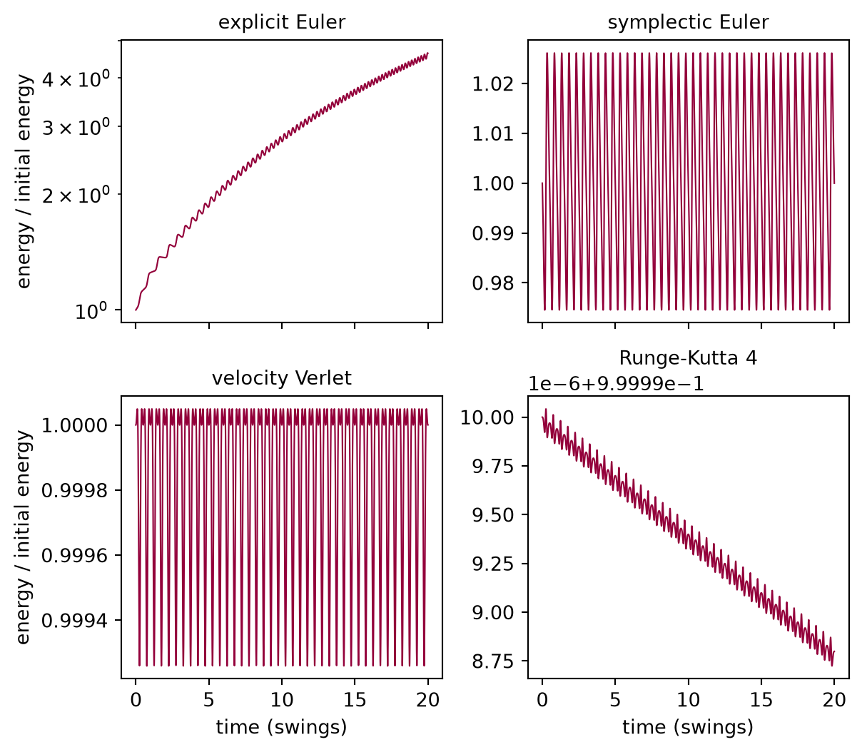
From here on the amplitude is 120°, well beyond the small-angle regime, where no formula gives the motion. The cell runs twenty swings with each of the four methods at 100 steps per small-angle period and reports the drift of the energy.

amplitude = 120  # degrees
swing = pendulum_period(length, np.radians(amplitude))

src/pbc/mechanics/experiments/energy_conservation.py, lines 45 to 46, read from the repository when this page was built.

def twenty_swings(experiment: Experiment) -> dict:
    """Twenty swings at the amplitude of the example with each method;
    record the table of the energy drift and return the runs."""
    runs = {
        integrator.name: run_swings(integrator, amplitude, 100, 20)
        for integrator in INTEGRATORS
    }

    rows = []
    for integrator in INTEGRATORS:
        energies = mechanical_energy(runs[integrator.name], mass, potential)
        rows.append(
            (integrator.name, energy_drift(energies), energies[-1] / energies[0])
        )

    experiment.table(
        "twenty-swings",
        rows,
        columns=[
            ("method", "", ""),
            ("energy drift", "", ".1e"),
            ("energy at the end / initial", "", ".4f"),
        ],
        caption="Drift of the energy over twenty swings at the amplitude of the "
        "example, and the energy at the end relative to the start.",
    )
    return runs

src/pbc/mechanics/experiments/energy_conservation.py, lines 171 to 197, read from the repository when this page was built.

Drift of the energy over twenty swings at the amplitude of the example, and the energy at the end relative to the start.

method	energy drift	energy at the end / initial
explicit Euler	3.6e+00	4.6331
symplectic Euler	2.6e-02	1.0000
velocity Verlet	7.4e-04	1.0000
Runge-Kutta 4	1.3e-06	1.0000

The period of this swing is 2.7546 s, or 1.3729 small-angle periods, and the run takes 2746 steps of 0.02006 s.

def draw_pendulum_energy(runs: dict) -> Figure:
    """The energy over twenty swings for each method."""
    fig, axes = plt.subplots(2, 2, figsize=(6.4, 5.6), sharex=True)
    for ax, integrator in zip(axes.flat, INTEGRATORS, strict=True):
        trajectory = runs[integrator.name]
        energies = mechanical_energy(trajectory, mass, potential)
        ax.plot(
            trajectory.t / swing, energies / energies[0], color="#93003a", linewidth=0.8
        )
        if integrator.name == "explicit Euler":
            ax.set_yscale("log")
        ax.set_title(integrator.name, fontsize=10)
    for ax in axes[1]:
        ax.set_xlabel("time (swings)")
    for ax in axes[:, 0]:
        ax.set_ylabel("energy / initial energy")
    fig.tight_layout()
    return fig

src/pbc/mechanics/experiments/energy_conservation.py, lines 200 to 217, read from the repository when this page was built.

Figure 3: simulated Explicit Euler lets the energy grow without limit, the two symplectic methods keep it in a band that repeats every swing, and the classical Runge-Kutta method loses a little at every step. Each panel has its own vertical scale, so the sizes of the bands are in the table, not in the figure.

    euler_ratio = mechanical_energy(runs["explicit Euler"], mass, potential)
    euler_ratio = euler_ratio[-1] / euler_ratio[0]

src/pbc/mechanics/experiments/energy_conservation.py, lines 520 to 521, read from the repository when this page was built.

Numerically verified (pendulum at the amplitude and the step of the example): The four behaviours are the ones the previous lesson derived on the oscillator, on a force for which nothing can be derived in closed form: explicit Euler has multiplied the energy by 4.6 in twenty swings, the two symplectic methods stay in bands that do not widen, and the classical Runge-Kutta method loses a little at every step. The oscillator result is therefore not a special property of the linear force. Now halve the step. The cell repeats the twenty swings at 50, 100, 200, and 400 steps per small-angle period, and the observed order is the logarithm to base two of the ratio of successive drifts.

step_counts = [50, 100, 200, 400]

src/pbc/mechanics/experiments/energy_conservation.py, line 49, read from the repository when this page was built.

def drift_orders(experiment: Experiment) -> dict:
    """The energy drift over twenty swings for each method and step count,
    with the observed order; record the table and return the drifts."""
    drifts = {
        integrator.name: np.array(
            [
                energy_drift(
                    mechanical_energy(
                        run_swings(integrator, amplitude, n, 20), mass, potential
                    )
                )
                for n in step_counts
            ]
        )
        for integrator in INTEGRATORS
    }

    rows = []
    columns = [("steps per T0", "", "d")]
    for integrator in INTEGRATORS:
        columns += [(f"{integrator.name}: drift", "", ".1e"), ("order", "", ".2f")]
    for i, n in enumerate(step_counts):
        row = [n]
        for integrator in INTEGRATORS:
            drift = drifts[integrator.name]
            row += [drift[i], np.log2(drift[i - 1] / drift[i]) if i else None]
        rows.append(row)

    experiment.table(
        "drift-orders",
        rows,
        columns=columns,
        caption="Energy drift over twenty swings against the number of steps per "
        "small-angle period, with the observed order, to two significant digits.",
    )
    return drifts

src/pbc/mechanics/experiments/energy_conservation.py, lines 220 to 255, read from the repository when this page was built.

Energy drift over twenty swings against the number of steps per small-angle period, with the observed order, to two significant digits.

steps per T0	explicit Euler: drift	order	symplectic Euler: drift	order	velocity Verlet: drift	order	Runge-Kutta 4: drift	order
50	7.3e+00		5.3e-02		3.0e-03		3.9e-05
100	3.6e+00	1.00	2.6e-02	1.02	7.4e-04	2.00	1.3e-06	4.95
200	1.8e+00	1.02	1.3e-02	1.01	1.9e-04	2.00	4.2e-08	4.91
400	8.9e-01	1.01	6.5e-03	1.00	4.6e-05	2.00	1.5e-09	4.85

Numerically verified (pendulum at the amplitude of the example, over the four steps of the table): The drift of the two first-order methods halves with the step, the drift of velocity Verlet falls by the factor of the second order, and the drift of the classical Runge-Kutta method falls by about 30 when the step halves: the observed order of that method is about 4.9, more than its order. For the oscillator the previous lesson derived that one step multiplies the energy by a factor that differs from one by a power of the step one higher than the order of the method, and a number of steps proportional to the inverse step then gives the power the table shows. The pendulum has the same pattern, but for it the lesson only measures it. The orders are those of the methods, or better, measured without a formula for the motion. This is the convergence test for a force without a closed form, and the drift at the finest step is the accuracy of the energy the run can claim.

One step of explicit Euler

The explanation derived the energy that one step of explicit Euler adds, $\tfrac12\Delta t^2 (m a^2 + U'' v^2)$. The cell compares it with the program for three states of the true motion at the amplitude of the examples, chosen by the energy: the release, the state at the height of a right angle, and the bottom. It does so at the step of the runs, at half that step, and at a quarter of it.

def step_energy_gain(experiment: Experiment) -> list:
    """The energy one explicit Euler step gains at three angles and three
    steps, against the formula; record the table and return its rows."""
    dt = t0 / 100
    total = mass * g * length * (1 - np.cos(np.radians(amplitude)))  # J
    rows = []
    for degrees in (amplitude, 60, 0):
        theta = np.radians(degrees)
        speed = np.sqrt(2 * (total - mass * g * length * (1 - np.cos(theta))) / mass)
        state = State(t=0.0, x=[length * theta], v=[speed])
        acceleration = -g * np.sin(theta)
        curvature = mass * g / length * np.cos(theta)  # U'' in J/m^2
        row = [degrees, speed]
        for step in (dt, dt / 2, dt / 4):
            gain = mechanical_energy(
                simulate(state, pendulum, step, 1, step=euler.step), mass, potential
            )
            formula = 0.5 * step**2 * (mass * acceleration**2 + curvature * speed**2)
            row += [gain[1] - gain[0], (gain[1] - gain[0]) / formula - 1]
        rows.append(row)

    experiment.table(
        "step-energy-gain",
        rows,
        columns=[("angle", "degrees", "d"), ("speed", "m/s", ".3f")]
        + [
            (f"gain at {label}", "J", ".3e")
            if k == 0
            else (f"difference at {label}", "", ".1e")
            for label in ("the step", "half", "a quarter")
            for k in (0, 1)
        ],
        caption="Energy gained in one explicit Euler step, and its relative "
        "difference from the formula, at the step, half of it, and a quarter "
        "of it.",
    )
    return rows

src/pbc/mechanics/experiments/energy_conservation.py, lines 258 to 294, read from the repository when this page was built.

Energy gained in one explicit Euler step, and its relative difference from the formula, at the step, half of it, and a quarter of it.

angle (degrees)	speed (m/s)	gain at the step (J)	difference at the step	gain at half (J)	difference at half	gain at a quarter (J)	difference at a quarter
120	0.000	1.452e-02	-2.2e-14	3.630e-03	-2.2e-14	9.074e-04	4.7e-13
60	4.429	3.287e-02	-3.0e-02	8.344e-03	-1.5e-02	2.102e-03	-7.4e-03
0	5.424	5.802e-02	-9.9e-04	1.451e-02	-2.5e-04	3.629e-03	-6.2e-05

Numerically verified (explicit Euler on the pendulum, three states of the motion of the examples): The formula gives the energy gain of one step to the leading order: the relative difference is at most 3e-02 over the table, and falls as the step falls, from -3.0e-02 to -7.4e-03 at the state of the right angle, as the neglected term of the next order in $\Delta t$ requires. At the release, the state of rest, the gain is positive although the velocity is zero, because the first term does not need a velocity.

What the energy does not see

Velocity Verlet keeps the energy within a band of 7e-04 over the twenty swings of the run, and the band is no wider at the end than at the start. Is the simulated motion right to that accuracy? The cell measures, for the three stable methods at the step of the runs, the time of each forward passage through the bottom, and reports how far behind or ahead of the exact period the passages fall as the swings go by.

def period_lag(experiment: Experiment, runs: dict) -> list:
    """The lag of the bob behind the exact period at its forward passages
    for the methods after explicit Euler; record the table and return its
    rows."""
    rows = []
    for integrator in INTEGRATORS[1:]:
        trajectory = runs[integrator.name]
        crossings = forward_crossings(trajectory)
        lag = crossings - (crossings[0] + np.arange(len(crossings)) * swing)
        drift = energy_drift(mechanical_energy(trajectory, mass, potential))
        rows.append(
            (integrator.name, drift, 1e3 * lag[5], 1e3 * lag[10], 1e3 * lag[19])
        )

    experiment.table(
        "period-lag",
        rows,
        columns=[
            ("method", "", ""),
            ("energy drift", "", ".1e"),
            ("lag after 5 swings", "ms", ".2f"),
            ("lag after 10 swings", "ms", ".2f"),
            ("lag after 19 swings", "ms", ".2f"),
        ],
        caption="Time by which the bob is behind (positive) or ahead of "
        "(negative) the exact period at its forward passages through the "
        "bottom, with the energy drift of the run.",
    )
    return rows

src/pbc/mechanics/experiments/energy_conservation.py, lines 297 to 325, read from the repository when this page was built.

Time by which the bob is behind (positive) or ahead of (negative) the exact period at its forward passages through the bottom, with the energy drift of the run.

method	energy drift	lag after 5 swings (ms)	lag after 10 swings (ms)	lag after 19 swings (ms)
symplectic Euler	2.6e-02	1.13	2.27	4.31
velocity Verlet	7.4e-04	-0.98	-1.97	-3.74
Runge-Kutta 4	1.3e-06	0.00	-0.01	-0.02

    bottom_speed = np.sqrt(2 * g * length * (1 - np.cos(np.radians(amplitude))))

src/pbc/mechanics/experiments/energy_conservation.py, line 542, read from the repository when this page was built.

Numerically verified (the three stable methods, the amplitude and the step of the example): The lag grows in proportion to the number of swings for every method: the simulated period differs from the exact one by a fixed fraction, and the error accumulates. For velocity Verlet the energy band is 35 times narrower than that of symplectic Euler, and the lag is about the same size with the opposite sign. After the last passage both bobs are off in time, by 4.3 ms and 3.7 ms, which at the bottom, where the bob moves at 5.4 m/s, is a position error of 2.3 cm for symplectic Euler, with the energy correct to the drift of the table. The energy band bounds the error in the energy and nothing else. Only a comparison in time, here against the exact period, can see a phase error.

Over the top

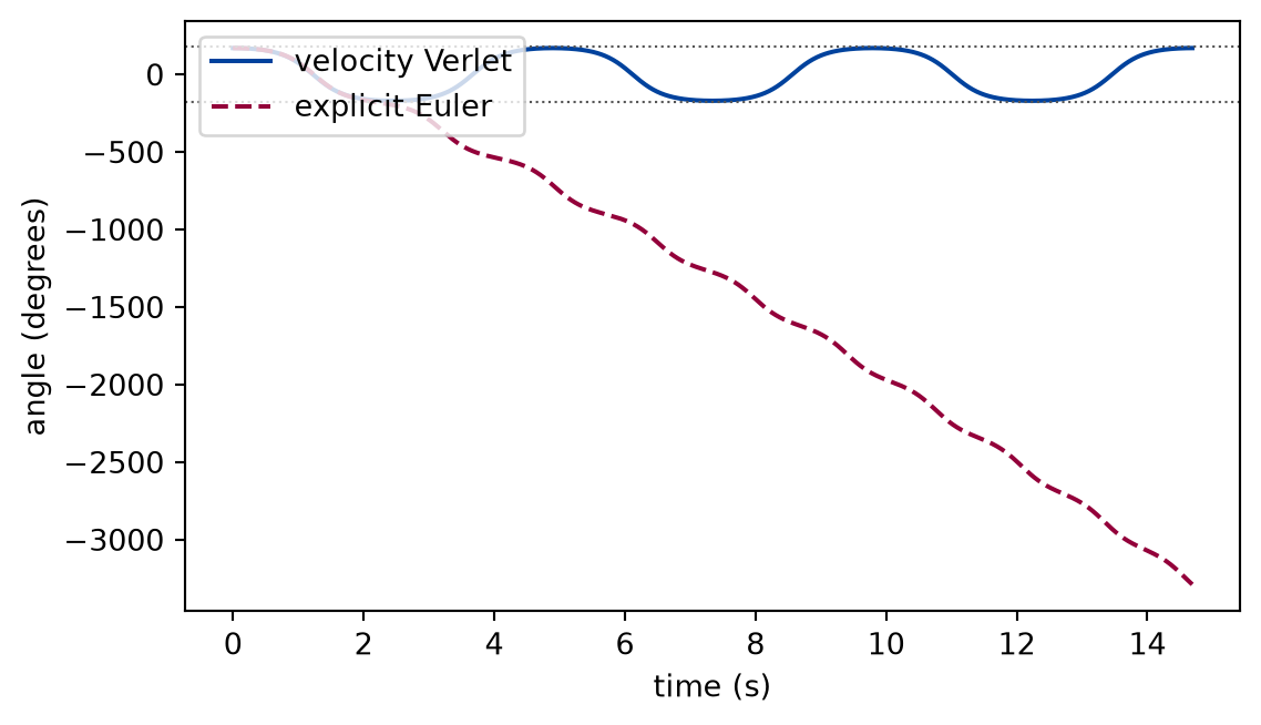
Released from rest at 170°, the pendulum has 0.9924 of the energy $2 m g L$ it would need to reach the top, so the true motion swings back and forth forever between $\pm 170°$. The cell runs three swings with explicit Euler and with velocity Verlet at 200 steps per small-angle period and reports the largest energy and the largest angle each one reaches.

def near_the_top(experiment: Experiment):
    """Three swings of the pendulum released at 170 degrees with explicit
    Euler and velocity Verlet; record the table and return the runs, its
    rows, and the energy of the top, in J."""
    separatrix = 2 * mass * g * length  # the energy at the top, J
    runs = {
        integrator.name: run_swings(integrator, 170, 200, 3)
        for integrator in (euler, verlet)
    }

    rows = []
    for integrator in (euler, verlet):
        trajectory = runs[integrator.name]
        energies = mechanical_energy(trajectory, mass, potential)
        largest_angle = np.degrees(np.max(np.abs(trajectory.x[:, 0])) / length)
        rows.append(
            (
                integrator.name,
                energies[0] / separatrix,
                np.max(energies) / separatrix,
                largest_angle,
            )
        )

    experiment.table(
        "near-the-top",
        rows,
        columns=[
            ("method", "", ""),
            ("initial energy / top", "", ".4f"),
            ("largest energy / top", "", ".4f"),
            ("largest angle", "degrees", ".0f"),
        ],
        caption="The energy, in units of the energy of the top, and the largest "
        "angle that each method reaches in three swings of the pendulum "
        "released near the top.",
    )
    return runs, rows, separatrix

src/pbc/mechanics/experiments/energy_conservation.py, lines 328 to 365, read from the repository when this page was built.

The energy, in units of the energy of the top, and the largest angle that each method reaches in three swings of the pendulum released near the top.

method	initial energy / top	largest energy / top	largest angle (degrees)
explicit Euler	0.9924	1.3224	3289
velocity Verlet	0.9924	0.9924	170

def over_the_top(runs: dict, separatrix: float):
    """When explicit Euler's energy passes the top and when its angle does,
    in s."""
    euler_energies = mechanical_energy(runs["explicit Euler"], mass, potential)
    trajectory = runs["explicit Euler"]
    crossed = trajectory.t[np.argmax(euler_energies > separatrix)]
    past_top = trajectory.t[np.argmax(np.abs(trajectory.x[:, 0]) / length > np.pi)]
    return crossed, past_top

src/pbc/mechanics/experiments/energy_conservation.py, lines 368 to 375, read from the repository when this page was built.

    crossed, past_top = over_the_top(top_runs, separatrix)
    swing_170 = pendulum_period(length, np.radians(170))

src/pbc/mechanics/experiments/energy_conservation.py, lines 561 to 562, read from the repository when this page was built.

def draw_pendulum_over_the_top(runs: dict) -> Figure:
    """The angle against time near the top, explicit Euler and Verlet."""
    fig, ax = plt.subplots(figsize=(6.4, 3.6))
    for integrator, style in ((verlet, "-"), (euler, "--")):
        trajectory = runs[integrator.name]
        ax.plot(
            trajectory.t,
            np.degrees(trajectory.x[:, 0] / length),
            color="#00429d" if integrator is verlet else "#93003a",
            linestyle=style,
            label=integrator.name,
        )
    ax.axhline(180, color="#555555", linewidth=0.8, linestyle=":")
    ax.axhline(-180, color="#555555", linewidth=0.8, linestyle=":")
    ax.set_xlabel("time (s)")
    ax.set_ylabel("angle (degrees)")
    ax.legend(loc="upper left")
    return fig

src/pbc/mechanics/experiments/energy_conservation.py, lines 378 to 395, read from the repository when this page was built.

Figure 4: simulated Explicit Euler does not turn back at the far end: it winds round and round, a motion that the pendulum with this energy cannot have, while velocity Verlet swings between the two release angles.

Explicit Euler adds energy at every step, by the amount the previous example checked, and at this step the energy of the top is reached after 1.07 s, which is 0.88 of the time the true bob needs for the quarter swing down to the bottom. Numerically verified (explicit Euler, the step and the release of this example): From there the simulation describes a rotating pendulum, a different motion from the one that was asked for: the angle passes the top at 2.22 s, later than the energy, and ends at 3289°. The error is not a digit; it is the kind of motion. The energy crossed its line before the angle crossed the top, and it is the cheaper of the two to watch, because it needs no exact solution and no knowledge of where the top is.

Limits

What this lesson shows holds for a single conservative force, one degree of freedom, and four fixed-step methods.

• The energy checks the motion only up to a phase. The lag table shows a small energy drift next to a position error that grows with every swing; an exact period, or another independent quantity, is needed to see it.
• The bands of the symplectic methods are measured for twenty swings at the steps of the tables. The theory that would extend them to longer runs, or to steps outside the stable range, is not derived here, and the oscillator derivation of the previous lesson does not carry over to the pendulum in general.
• The observed order of the classical Runge-Kutta method is measured on one amplitude. Why it is about five, not four, is derived for the oscillator only.
• The energy of the explicit Euler step is a leading-order formula, checked at three states; it does not bound the drift of a run.
• Round-off is not what limits the results: the smallest drift of the tables, 1.5e-09, is 7e+06 times the spacing of double-precision numbers at one. A finer step or a longer run would reach the region where it matters.
• The pendulum has one degree of freedom, and the exact period is the only exact result. With several bodies, later in the course, no such formula exists and the energy is one of several conserved quantities.
• A force that depends on the velocity, as the drag of the second exercise does, has no conserved energy; the energy balance of that exercise holds to the accuracy of the method, as the exercise measures.

Self-check. Two runs of the same pendulum keep the energy within bands of equal width over a thousand swings. A colleague concludes that they simulate the motion equally well. Is that right? Say what you would compute to find out, and what the lag table of this lesson shows about it.

With scripts, you can record in this browser that you answered this question.

Solution to the self-check

No. The energy fixes how fast the bob moves at each angle, not where in the swing it is at a given time. A method can leave the energy curve almost alone and still turn the state along it too fast or too slowly, so the simulated bob drifts away from the true one in time. The lag table shows it: velocity Verlet has an energy band 35 times narrower than that of symplectic Euler, and a lag of about the same size. To tell the two runs apart, compare a quantity that depends on time, such as the times of the passages through the bottom against the exact period, which this lesson did, or the two runs against each other at the same time. The assumption that fails is the one about what the energy measures: it is one necessary condition on the motion, not a statement that the motion is right.

Exercises

Exercise 1. One per cent. At what amplitude does the period exceed the small-angle period by one per cent? Estimate it from the series $T \approx T_0\,(1 + \theta_0^2/16)$, find it from the exact period, and confirm it with a simulation.

Solution to exercise 1

The series gives $\theta_0^2/16 = 0.01$, so $\theta_0 = 0.4$ rad. The exact amplitude is where pendulum_period equals $1.01\,T_0$, found by a root finder; the simulation measures the period as in the first example. Adding the $\theta_0^4$ term to the series, as the explanation derived it, shows where the difference between the first two answers comes from.

def one_per_cent_longer(experiment: Experiment):
    """Exercise 1: the amplitude at which the period is one per cent above
    the small-angle period, from the series, exactly, and simulated; record
    the table."""
    from_series = np.degrees(np.sqrt(0.16))
    two_terms = np.degrees(
        brentq(lambda a: a**2 / 16 + 11 * a**4 / 3072 - 0.01, 0.01, 1.0)
    )
    exact_amplitude = brentq(
        lambda angle: pendulum_period(length, angle) / t0 - 1.01, 0.01, 1.0
    )
    measured = np.mean(
        np.diff(forward_crossings(run_swings(rk4, np.degrees(exact_amplitude), 200, 3)))
    )

    experiment.table(
        "one-per-cent-longer",
        [
            ("one-term series", from_series, None),
            ("two-term series", two_terms, None),
            ("exact period", np.degrees(exact_amplitude), None),
            (
                "simulation at the exact amplitude",
                np.degrees(exact_amplitude),
                measured / t0,
            ),
        ],
        columns=[
            ("source", "", ""),
            ("amplitude", "degrees", ".2f"),
            ("period / T0", "", ".4f"),
        ],
        caption="Amplitude at which the period exceeds the small-angle period by "
        "one per cent, to two decimals, and the simulated period there.",
    )
    return from_series, two_terms, exact_amplitude

src/pbc/mechanics/experiments/energy_conservation.py, lines 398 to 433, read from the repository when this page was built.

Amplitude at which the period exceeds the small-angle period by one per cent, to two decimals, and the simulated period there.

source	amplitude (degrees)	period / T0
one-term series	22.92
two-term series	22.81
exact period	22.81
simulation at the exact amplitude	22.81	1.0100

About 23°. The one-term series is 0.104° above the exact amplitude, and the second term of the series reduces that to 0.001°, which is what the first term leaves out. A pendulum clock keeps its amplitude small for this reason, and keeps it constant because even a small amplitude that varied would vary the period.

Exercise 2. The energy balance with drag. Add linear drag with the constant $b = 0.1$ kg/s to the pendulum released at 120°. The energy is no longer conserved; the work-energy theorem says that what is lost equals the work done by the drag, $W = -\int b\,v^2\,\mathrm{d}t$. Run five swings with velocity Verlet at 100, 200, and 400 steps per small-angle period, compute both sides, and compare the gap between them with the drift of the undamped run at the same step.

Solution to exercise 2

The drag model of the Newton’s laws lesson plugs into newton next to the pendulum force. The work is the integral of the power $-b\,v^2$ over the run, by the trapezoidal rule on the simulated velocities.

def damped_budget(experiment: Experiment, drifts: dict) -> None:
    """Exercise 2: the energy lost to a linear drag against the work the
    drag does over five swings; record the table."""
    b = 0.1  # kg/s
    damped = newton(mass, pendulum_force(mass, length), linear_drag(b))

    rows = []
    for n in step_counts[1:]:
        trajectory = simulate(
            released(amplitude),
            damped,
            t0 / n,
            round(5 * swing / t0 * n),
            step=verlet.step,
        )
        energies = mechanical_energy(trajectory, mass, potential)
        power = -b * np.sum(trajectory.v**2, axis=1)
        work = np.trapezoid(power, trajectory.t)
        rows.append(
            (
                n,
                energies[0] - energies[-1],
                -work,
                energies[0] - energies[-1] + work,
                drifts["velocity Verlet"][step_counts.index(n)],
            )
        )

    experiment.table(
        "damped-budget",
        rows,
        columns=[
            ("steps per T0", "", "d"),
            ("energy lost", "J", ".4f"),
            ("work by drag", "J", ".4f"),
            ("gap", "J", ".1e"),
            ("undamped drift", "", ".1e"),
        ],
        caption="Energy lost, work done by the drag, and the gap between them "
        "over five swings, with the drift of the undamped run at the same step.",
    )

src/pbc/mechanics/experiments/energy_conservation.py, lines 436 to 476, read from the repository when this page was built.

Energy lost, work done by the drag, and the gap between them over five swings, with the drift of the undamped run at the same step.

steps per T0	energy lost (J)	work by drag (J)	gap (J)	undamped drift
100	10.6334	10.6201	1.3e-02	7.4e-04
200	10.6320	10.6287	3.3e-03	1.9e-04
400	10.6315	10.6307	8.3e-04	4.6e-05

The budget closes to the accuracy of the method: the gap quarters when the step halves, like the drift of the undamped run, and is of the same order as that drift times the initial energy. With a non-conservative force the check is the balance rather than the conservation, and it is just as sharp.

Exercise 3. The step for a stated drift. How many steps per small-angle period does velocity Verlet need to keep the energy drift of the 120° pendulum below $10^{-5}$? Predict the number from the convergence table, then run fifty swings with it.

Solution to exercise 3

The drift of a second-order method is proportional to $\Delta t^2$, so the step for the drift $\delta$ is the step of a run with the drift $\delta_1$ times $\sqrt{\delta / \delta_1}$. The run at 100 steps per period is the reference. The band of a symplectic method does not widen with the run in the runs of this lesson, so the prediction is tested for fifty swings as for twenty.

def steps_for_a_drift(experiment: Experiment, drifts: dict) -> None:
    """Exercise 3: the steps per small-angle period that velocity Verlet
    needs for a drift of 1e-5 over fifty swings; record the table."""
    target = 1e-5
    needed = int(np.ceil(100 * np.sqrt(drifts["velocity Verlet"][1] / target)))
    trajectory = run_swings(verlet, amplitude, needed, 50)
    drift = energy_drift(mechanical_energy(trajectory, mass, potential))

    experiment.table(
        "steps-for-a-drift",
        [(needed, drift, len(trajectory.t) - 1)],
        columns=[
            ("steps per T0", "", "d"),
            ("drift over fifty swings", "", ".2e"),
            ("steps in the run", "", "d"),
        ],
        caption="The predicted number of steps per small-angle period, and the "
        "drift of the run that uses it.",
    )

src/pbc/mechanics/experiments/energy_conservation.py, lines 479 to 497, read from the repository when this page was built.

The predicted number of steps per small-angle period, and the drift of the run that uses it.

steps per T0	drift over fifty swings	steps in the run
861	9.99e-06	59103

The prediction lands on the target. The previous lesson’s rule stands: over a long run it is the symplectic method whose energy can be trusted, and the order tells the cost of the accuracy.

Run this experiment

This page was built from commit 6417e2ff90258bd2d2ba21d217eb7666fd24f680 of the repository.

In a clone at that commit, with the project’s Python packages installed, this command runs the experiment of this page:

uv run --locked --no-dev python -m pbc.mechanics.experiments.energy_conservation results

Files, tests, and every command

The files behind it:

• site/lessons/mechanics/06-energy-conservation/index.qmd: this page, with every code cell.
• src/pbc/mechanics/dynamics.py: code the experiment runs.
• src/pbc/mechanics/integrators.py: code the experiment runs.
• src/pbc/mechanics/energy.py: code the experiment runs.
• src/pbc/mechanics/pendulum.py: code the experiment runs.
• src/pbc/mechanics/drag.py: code the experiment runs.
• src/pbc/mechanics/experiments/energy_conservation.py: code the experiment runs.
• src/pbc/experiment.py: code the experiment runs.
• tests/unit/test_dynamics.py: tests of that code.
• tests/unit/test_integrators.py: tests of that code.
• tests/unit/test_energy.py: tests of that code.
• tests/unit/test_pendulum.py: tests of that code.
• tests/unit/test_drag.py: tests of that code.
• tests/unit/test_energy_conservation_experiment.py: tests of that code.

With Git and uv installed (see the setup page), run:

git clone https://github.com/taspinar/physics-by-construction.git
cd physics-by-construction
git checkout 6417e2ff90258bd2d2ba21d217eb7666fd24f680
uv sync --locked --no-dev
uv run --locked --no-dev python -m pbc.mechanics.experiments.energy_conservation results

The experiment writes every figure of this page into results/, as <label>.png, and every number and table of the page, as the page shows it, into results/results.json. Its numbers match this page to the digits shown, and its figure files are the ones the page shows; digits beyond those can differ between machines, because floating-point libraries differ. Change the code of the experiment and run it again to see what changes.