Numerical integrators

Explicit Euler, symplectic Euler, velocity Verlet, and Runge-Kutta 4 behind one stepping interface, compared on the harmonic oscillator for accuracy, energy behaviour, and cost, so that a later simulation can choose its method for what it has to be trusted for.

Course

Classical mechanics, lesson 5 of 28

Slot

M5, Numerical integrators

Methods

Simulation

Difficulty

Intermediate, level 2 of 3

What you’ll learn

• Step a system with explicit Euler, symplectic Euler, velocity Verlet, and Runge-Kutta 4 behind one interface
• Compare integrators for accuracy, energy behaviour, and cost
• Choose an integrator for what a simulation has to be trusted for

Prerequisites

The harmonic oscillator.

Before you begin

• Complex numbers: modulus, argument, and the exponential of an imaginary number
• Calculus: Taylor expansion to fourth order
• Linear algebra: the determinant and the trace of a two-by-two matrix

Related

What symplectic Euler conserves

Previous

The harmonic oscillator

Next

Energy conservation

With scripts, this page keeps a record in your browser of whether you completed the lesson. Nothing is stored without them.

With scripts, this place suggests what to do next, with the reason, from the progress saved in your browser. Without them, follow the learning path.

A planet followed for a million orbits, a molecule followed for a million vibrations, a satellite predicted for years: each is a simulation that takes a very large number of small steps, and each step makes a small error that the next step inherits. How large the error is after a few steps is only half of the question. The other half is what the errors do when there are very many of them: whether the energy of the system grows, decays, or stays near where it began, because a planet that gains energy at every orbit does not stay in the solar system the simulation describes.

Every lesson so far has used explicit Euler, and the last one computed exactly how it fails on an oscillator: the energy is multiplied by the factor $1 + \omega^2 \Delta t^2$ at every step, and holding it to one per cent for ten periods took an impractical number of steps per period. The stepping interface of the Newton’s laws lesson was built for this moment. This lesson adds three methods behind it, each a function with the same signature, and compares all four on the harmonic oscillator, where the exact motion and the exact energy are known.

Three questions decide which method a simulation should use. How fast does the error shrink when the step shrinks: the order of the method. What does the method do to the energy over a long run: does it grow, decay, or stay within a band. What does a step cost, in evaluations of the force. The answers differ by method, and they are not a ranking: a method that is best for an accurate position after two periods is not the one to trust with the energy over a thousand. The lesson ends with the rule that follows.

Assumptions

The model and the program rest on these assumptions. Each one names what goes wrong when it does not hold.

1. The harmonic oscillator of the previous lesson. The same assumptions apply: Hooke’s law, no drag, a point mass, constant $m$ and $k$. The energy results below are exact for this force because the equations are linear. For a nonlinear force, such as the pendulum of the next lesson, the per-step factors and the conserved quantities are no longer closed formulas, and this lesson does not demonstrate how the energy behaves.
2. The step is below the stability limit of the method. Each method except explicit Euler has a largest step for which the oscillator stays bounded; the limits are derived below and tested in the first exercise. Above its limit a method amplifies the state at every step, and its order says nothing.
3. A smooth force. The orders are those for a force with enough derivatives. A force with a kink or a jump, such as a bounce, lowers the order of every method to first order unless the step lands on the event.
4. A force that does not depend on the velocity, for the energy results. The order results hold with a velocity-dependent force as well, as the second exercise checks, but “symplectic” is a property of a method on a conservative system; with drag there is no energy to conserve, and the velocity Verlet step evaluates the new acceleration at a predicted velocity.
5. Cost means evaluations of the acceleration. The wall-clock time of a step depends on the machine, the language, and what else it is doing, and it would change from build to build. The number of times a step calls the force function depends on nothing but the method, and for every simulation in which the force dominates the cost it is the right measure. The simple arithmetic around the calls is ignored.
6. Round-off is negligible. The errors of the accuracy table stay far above double-precision round-off, which is about $10^{-16}$ relative to the size of the numbers. Refining the fourth-order method much further would make its error grow again, from round-off, not from the method.
7. The methods are the fixed-step ones. Every step has the same length. The adaptive Runge-Kutta pair of SciPy’s solve_ivp (RK45) chooses its step from an error estimate and is a different stepper; nothing in this lesson measures it.

Four update rules

All four methods advance the state $(x_n, v_n)$ at time $t_n$ by one step $\Delta t$ to $(x_{n+1}, v_{n+1})$, using the acceleration function $a(t, x, v)$ of the model, and nothing else. For the oscillator $a = -\omega^2 x$. Each rule below answers one question: where should the rates of change be taken, so that the step follows the true motion as closely as possible for the number of times the force has to be evaluated.

Explicit Euler, as before: both rates are taken at the start of the step.

$$x_{n+1} = x_n + v_n\,\Delta t, \qquad v_{n+1} = v_n + a(t_n, x_n, v_n)\,\Delta t.$$

It follows the Taylor expansion of the exact motion only through the term in $\Delta t$, and misses $\tfrac12 a\,\Delta t^2$ in the position, which is why it has order one.

Symplectic Euler changes one thing: the velocity is updated first, and the new velocity moves the particle. This is the velocity-first ordering; updating the position first, with the old velocity, is explicit Euler.

$$v_{n+1} = v_n + a(t_n, x_n, v_n)\,\Delta t, \qquad x_{n+1} = x_n + v_{n+1}\,\Delta t.$$

It costs exactly as much as explicit Euler and has the same order, and it does something entirely different to the energy, as the examples show.

Velocity Verlet moves the position with the Taylor expansion to second order, then changes the velocity by the average of the acceleration at the start and at the end of the step, a trapezoid in place of the rectangle that Euler uses.

$$x_{n+1} = x_n + v_n\,\Delta t + \tfrac{1}{2}\,a_n\,\Delta t^2, \qquad v_{n+1} = v_n + \tfrac{1}{2}\,(a_n + a_{n+1})\,\Delta t,$$

with $a_n = a(t_n, x_n, v_n)$ and $a_{n+1} = a(t_{n+1}, x_{n+1}, \cdot)$. When the force does not depend on the velocity, the dot is immaterial, and $a_{n+1}$ can be carried over to the next step, so the method costs one evaluation per step. The stepping interface keeps nothing between steps, so the implementation below evaluates twice, with the explicit Euler prediction $v_n + a_n \Delta t$ in place of the dot.

Classical Runge-Kutta (the fourth-order method with a fixed step) evaluates the rates four times, at the start, twice at the midpoint, and at the end of the step, each time at a state predicted with the rates found so far, and takes their weighted average. For the pair $y = (x, v)$ with the rate $f(t, y) = (v, a(t, x, v))$,

$$\begin{aligned} k_1 &= f(t_n, y_n), & k_2 &= f\bigl(t_n + \tfrac{1}{2}\Delta t,\; y_n + \tfrac{1}{2}\Delta t\,k_1\bigr), \\ k_3 &= f\bigl(t_n + \tfrac{1}{2}\Delta t,\; y_n + \tfrac{1}{2}\Delta t\,k_2\bigr), & k_4 &= f\bigl(t_n + \Delta t,\; y_n + \Delta t\,k_3\bigr), \end{aligned} \qquad y_{n+1} = y_n + \tfrac{\Delta t}{6}\,(k_1 + 2k_2 + 2k_3 + k_4).$$

The weights are not arbitrary. When the rate does not depend on $y$ at all, $k_2 = k_3$ is the rate at the midpoint, and the step is $\tfrac{\Delta t}{6}(f_{\mathrm{start}} + 4 f_{\mathrm{mid}} + f_{\mathrm{end}})$: Simpson’s rule for the integral of the rate, which is exact for cubics. The extra evaluations make the same weights work when the rate depends on $y$, and the step agrees with the Taylor expansion of the exact motion through the fourth power of $\Delta t$. Showing that for a general rate takes several pages of algebra; the accuracy table below measures it instead.

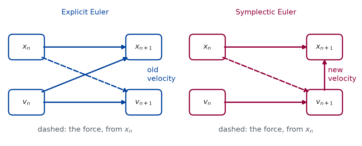
The two Euler rules differ only in an ordering, and a picture of the data flow shows what the ordering changes:

def draw_update_orderings() -> Figure:
    """The data flow of explicit and of symplectic Euler, as a sketch."""
    fig, axes = plt.subplots(1, 2, figsize=(6.4, 3.0))
    orderings = (
        ("Explicit Euler", 0, False),
        ("Symplectic Euler", 1, True),
    )
    for ax, (name, colour, velocity_first) in zip(axes, orderings, strict=True):
        diagrams.frame(ax, (-0.2, 4.4), (-0.7, 3.2))
        diagrams.text(ax, (2.1, 3.0), name, colour=colour)
        left, right = 0.4, 3.8
        diagrams.state_box(
            ax, (left, 2.0), "$x_n$", width=1.0, height=0.7, colour=colour
        )
        diagrams.state_box(
            ax, (left, 0.4), "$v_n$", width=1.0, height=0.7, colour=colour
        )
        diagrams.state_box(
            ax, (right, 2.0), "$x_{n+1}$", width=1.0, height=0.7, colour=colour
        )
        diagrams.state_box(
            ax, (right, 0.4), "$v_{n+1}$", width=1.0, height=0.7, colour=colour
        )
        diagrams.arrow(ax, (left + 0.5, 2.0), (right - 0.5, 2.0), colour=colour)
        diagrams.arrow(ax, (left + 0.5, 0.4), (right - 0.5, 0.4), colour=colour)
        diagrams.arrow(
            ax, (left + 0.45, 1.7), (right - 0.45, 0.7), colour=colour, linestyle="--"
        )
        if velocity_first:
            diagrams.arrow(ax, (right, 0.75), (right, 1.65), colour=colour)
            diagrams.text(
                ax, (right + 0.1, 1.2), "new\nvelocity", ha="left", colour=colour
            )
        else:
            diagrams.arrow(ax, (left + 0.45, 0.7), (right - 0.45, 1.7), colour=colour)
            diagrams.text(
                ax, (right + 0.1, 1.2), "old\nvelocity", ha="left", colour=colour
            )
        diagrams.text(
            ax, (2.1, -0.4), "dashed: the force, from $x_n$", colour="#57606a"
        )
    fig.tight_layout()
    return fig

src/pbc/mechanics/experiments/numerical_integrators.py, lines 61 to 103, read from the repository when this page was built.

Figure 1: conceptual The same four quantities, wired in two orders. In explicit Euler the position is moved by the old velocity, so the two updates are independent of each other. In symplectic Euler the velocity is updated first and the position is moved by the new one, so the position update waits for the velocity update.

The diagram is drawn by hand, and nothing in it is computed. It answers the question the two formulas raise: if both methods read the same inputs, why should they differ? The difference is a single arrow, the source of the velocity that moves the position, and the energy section below follows what that one arrow does.

Order of accuracy

A method whose single step matches the Taylor expansion of the motion through $\Delta t^p$ has a local error of order $\Delta t^{p+1}$ per step. Reaching a fixed time takes $t/\Delta t$ steps, so the global error at that time is of order $\Delta t^p$: the method has order $p$. Explicit and symplectic Euler have order one, velocity Verlet order two, and the classical Runge-Kutta method order four. The examples measure the orders the way the earlier lessons did, by halving the step and taking the binary logarithm of the ratio of successive errors.

The order is what a digit costs. Halving the step divides the error by $2^p$, so one more correct decimal digit costs a factor $10^{1/p}$ in the number of steps: ten times the steps for a first-order method, about three times for second order, less than twice for fourth. Over a few periods the fourth-order method wins by a wide margin, as the cost example shows.

What each method does to the energy

The accuracy question has a second side. A method with a small error after two periods may still drift away over a thousand, and whether it does is decided by what one step does to the energy, which for the oscillator can be computed exactly.

Write the state as the single complex number $u = v + i\,\omega x$. The reason is that the oscillator is a rotation: the equations of motion $\dot x = v$ and $\dot v = -\omega^2 x$ become the single equation $\dot u = i\omega u$, and the energy is $E = \tfrac{1}{2} m\,|u|^2$. The exact motion multiplies $u$ by $e^{i\omega\Delta t}$ per step, a pure rotation that keeps $|u|$ fixed. Explicit Euler and the classical Runge-Kutta method treat $x$ and $v$ alike, and on this linear system each of their steps multiplies $u$ by a polynomial in $z = \omega\,\Delta t$: explicit Euler by $1 + iz$, and Runge-Kutta by the Taylor polynomial of $e^{iz}$ to fourth order, $R(iz) = 1 + iz + \tfrac{(iz)^2}{2} + \tfrac{(iz)^3}{6} + \tfrac{(iz)^4}{24}$. The energy after a step is the energy before it times the squared modulus. For Runge-Kutta, collect the real and the imaginary part, $R(iz) = \bigl(1 - \tfrac{z^2}{2} + \tfrac{z^4}{24}\bigr) + i\bigl(z - \tfrac{z^3}{6}\bigr)$, and square both: the terms in $z^2$ and $z^4$ cancel, and what is left is

$$\frac{E_{n+1}}{E_n} = |1 + iz|^2 = 1 + z^2 \quad\text{(explicit Euler)}, \qquad \frac{E_{n+1}}{E_n} = |R(iz)|^2 = 1 - \frac{z^6}{72} + \frac{z^8}{576} \quad\text{(Runge-Kutta)}.$$

The first is the factor of the previous lesson. The second is below one for $z < 2\sqrt 2$: Runge-Kutta loses energy, by a tiny fixed fraction per step, $z^6/72$ for small $z$. The loss is steady, so it accumulates over a long run just as explicit Euler’s gain does, only far more slowly, and above $z = 2\sqrt 2$, fewer than about 2.2 steps per period, the factor exceeds one and the method is unstable.

Symplectic Euler and velocity Verlet treat $x$ and $v$ differently, so their step is not a multiplication of $u$ by a number, and the energy after a step is not a fixed multiple of the energy before. What decides their behaviour is the matrix that takes $(x_n, v_n)$ to $(x_{n+1}, v_{n+1})$. For the oscillator, substituting $a = -\omega^2 x$ into the update rules gives

$$M_{\mathrm{SE}} = \begin{pmatrix} 1 - z^2 & \Delta t \\ -\omega^2\Delta t & 1 \end{pmatrix}, \qquad M_{\mathrm{VV}} = \begin{pmatrix} 1 - \tfrac{z^2}{2} & \Delta t \\ -\omega^2\Delta t\,\bigl(1 - \tfrac{z^2}{4}\bigr) & 1 - \tfrac{z^2}{2} \end{pmatrix}.$$

Both have determinant exactly one, and trace $2 - z^2$. A determinant of one is the statement that the step preserves areas of phase space, as the true motion does; it is what the name symplectic stands for. It also fixes the behaviour of the state. A two-by-two matrix with determinant one has the eigenvalues $e^{\pm i\theta}$ with $2\cos\theta$ equal to its trace whenever the trace lies between $-2$ and $2$, and then the state is turned by the angle $\theta$ at every step on a closed curve, forever. That holds for $0 < z < 2$, so the stability limit of both methods is $z = 2$, fewer than $\pi$ steps per period. Beyond it the trace is below $-2$ and one eigenvalue has modulus greater than one. The limit itself is excluded: at $z = 2$ both eigenvalues are $-1$, the matrix cannot be diagonalised, and the state can grow in proportion to the number of steps.

The closed curve is an ellipse of a quadratic form that the step conserves exactly, a slightly different quantity from the energy:

$$\tilde E_{\mathrm{SE}} = \tfrac{1}{2} m \bigl(v^2 + \omega^2 x^2 - \omega^2 \Delta t\,x\,v\bigr), \qquad \tilde E_{\mathrm{VV}} = \tfrac{1}{2} m \Bigl(v^2 + \omega^2 \bigl(1 - \tfrac{1}{4}\omega^2 \Delta t^2\bigr)\,x^2\Bigr).$$

Each modified energy differs from the true one by a term of order $\Delta t$ (symplectic Euler) or $\Delta t^2$ (velocity Verlet) that oscillates with the motion. The computed state stays on the ellipse of its modified energy forever, so the true energy oscillates within a band of that width and never drifts out of it. The worked examples confirm that both are conserved to round-off. This is the property that makes these methods the choice for a long run: the energy error is bounded for all time, and not just small for a while.

Go deeper: Symplectic integrators (chapter 7 of Numerically Solving Ordinary Differential Equations) (Stuart Brorson, LibreTexts Mathematics, 7.2 Symplectic Euler and 7.3 Example, the simple harmonic oscillator; 7.4 and 7.5 on phase-space volume and Liouville's theorem; derivation.)

The same velocity-first rule, followed through the oscillator, and the reason a determinant of one means that phase-space area is preserved, in terms of Liouville’s theorem. The lesson does not need it: the matrix argument above is complete.

In short, for one step with $z = \omega\,\Delta t$:

• Explicit Euler. Order one, one evaluation per step. The energy is multiplied by $1 + z^2$. Stable for no step.
• Symplectic Euler. Order one, one evaluation per step. The energy is bounded; $\tilde E_{\mathrm{SE}}$ is conserved. Stable for $z < 2$.
• Velocity Verlet. Order two, two evaluations per step, or one with the acceleration carried over. The energy is bounded; $\tilde E_{\mathrm{VV}}$ is conserved. Stable for $z < 2$.
• Classical Runge-Kutta. Order four, four evaluations per step. The energy is multiplied by $1 - z^6/72 + z^8/576$. Stable for $z < 2\sqrt 2$.

Go deeper: Verlet Integration (Numerical Methods for Mechanics, 2023) (MIT course page "NMM 2023" (author not named on the page), Derivation, "As a Variation of Semi-Implicit Euler"; Properties, "Symplectic Properties"; derivation.)

Velocity Verlet seen as a half step of velocity-first symplectic Euler followed by a half step of its position-first counterpart, which explains why it keeps the bounded energy of symplectic Euler while gaining an order. Two half steps in the same ordering would not give it. The lesson does not need it.

The program

The three new steppers live in the module pbc.mechanics.integrators of the repository, next to the explicit Euler step of pbc.mechanics.dynamics, and all four go into simulate through its step argument. The listings in this section are read from the files when the site is built. Each marks the lines that carry the update order, because the order is what separates the methods.

def symplectic_euler_step(state: State, acceleration: Acceleration, dt: float) -> State:
    """Advance ``state`` by one symplectic Euler step of length ``dt`` (s).

    The velocity changes first, with the acceleration at the old state;
    then the *new* velocity moves the particle. One change of order against
    explicit Euler, with the same cost; it is the simplest method that keeps
    the energy of an oscillator bounded.
    """
    v = state.v + acceleration(state.t, state.x, state.v) * dt
    return State(t=state.t + dt, x=state.x + v * dt, v=v)

1. Line 24, v = state.v + acceleration(state.t, state.x, state.v) * dt: The velocity changes first, with the acceleration at the old state.
2. Line 25, return State(t=state.t + dt, x=state.x + v * dt, v=v): The new velocity, not the old one, moves the particle. This line is the whole difference from explicit Euler.

src/pbc/mechanics/integrators.py, lines 16 to 25, read from the repository when this page was built.

def verlet_step(state: State, acceleration: Acceleration, dt: float) -> State:
    """Advance ``state`` by one velocity Verlet step of length ``dt`` (s).

    The position moves by the Taylor expansion to second order, with the
    acceleration at the old state; the velocity changes by the average of
    the old acceleration and the one at the new position. When the force
    depends on the velocity, the new acceleration is evaluated at the
    explicit Euler prediction of the new velocity, which keeps the method
    second order.
    """
    a = acceleration(state.t, state.x, state.v)
    t = state.t + dt
    x = state.x + state.v * dt + 0.5 * a * dt**2
    a_next = acceleration(t, x, state.v + a * dt)
    return State(t=t, x=x, v=state.v + 0.5 * (a + a_next) * dt)

1. Line 40, x = state.x + state.v * dt + 0.5 * a * dt**2: The position takes the second-order Taylor term, with the acceleration at the old state.
2. Line 41, a_next = acceleration(t, x, state.v + a * dt): The second evaluation: at the new position, and at a predicted velocity, which is what keeps the order for a force that depends on the velocity.
3. Line 42, return State(t=t, x=x, v=state.v + 0.5 * (a + a_next) * dt): The velocity changes by the average of the two accelerations.

src/pbc/mechanics/integrators.py, lines 28 to 42, read from the repository when this page was built.

def rk4_step(state: State, acceleration: Acceleration, dt: float) -> State:
    """Advance ``state`` by one step of the classical fourth-order
    Runge-Kutta method, of length ``dt`` (s).

    The rates of change of position and velocity are evaluated four times:
    at the start of the step, twice at its midpoint, and at its end, each
    time at a state predicted with the rates found so far. The step uses
    their weighted average, which matches the Taylor expansion of the motion
    to fourth order.
    """
    t, x, v = state.t, state.x, state.v
    half = 0.5 * dt
    k1_x, k1_v = v, acceleration(t, x, v)
    k2_x = v + half * k1_v
    k2_v = acceleration(t + half, x + half * k1_x, k2_x)
    k3_x = v + half * k2_v
    k3_v = acceleration(t + half, x + half * k2_x, k3_x)
    k4_x = v + dt * k3_v
    k4_v = acceleration(t + dt, x + dt * k3_x, k4_x)
    return State(
        t=t + dt,
        x=x + dt / 6.0 * (k1_x + 2.0 * k2_x + 2.0 * k3_x + k4_x),
        v=v + dt / 6.0 * (k1_v + 2.0 * k2_v + 2.0 * k3_v + k4_v),
    )

1. Line 57, k1_x, k1_v = v, acceleration(t, x, v): The first rates, at the start of the step, as in explicit Euler.
2. Line 63, k4_v = acceleration(t + dt, x + dt * k3_x, k4_x): The last rates, at the end of the step, at the state predicted with the third rates.
3. Line 66, x=x + dt / 6.0 * (k1_x + 2.0 * k2_x + 2.0 * k3_x + k4_x),: The weights one, two, two, one over six: Simpson's rule when the rates do not depend on the state.

src/pbc/mechanics/integrators.py, lines 45 to 68, read from the repository when this page was built.

The four methods are listed with what the summary above says about them, so that an experiment can loop over them:

@dataclass(frozen=True)
class Integrator:
    """One method of the course: its stepper, with what to expect from it."""

    name: str
    step: Stepper
    # The error at a fixed time is proportional to dt ** order for a smooth
    # force and a step small enough for the method.
    order: int
    # Acceleration evaluations per step. The stepping interface keeps nothing
    # between steps, so velocity Verlet evaluates twice; a loop that carried
    # the last acceleration over would evaluate once.
    evaluations: int

src/pbc/mechanics/integrators.py, lines 71 to 83, read from the repository when this page was built.

def methods(experiment: Experiment) -> None:
    """Record the table of the four methods, as INTEGRATORS gives them."""
    experiment.table(
        "methods",
        [(i.name, i.step.__name__, i.order, i.evaluations) for i in INTEGRATORS],
        columns=[
            ("method", "", ""),
            ("stepper", "", ""),
            ("order", "", "d"),
            ("evaluations per step", "", "d"),
        ],
        caption="The four methods of the lesson, as the list INTEGRATORS gives them.",
    )

src/pbc/mechanics/experiments/numerical_integrators.py, lines 106 to 118, read from the repository when this page was built.

The four methods of the lesson, as the list INTEGRATORS gives them.

method	stepper	order	evaluations per step
explicit Euler	euler_step	1	1
symplectic Euler	symplectic_euler_step	1	1
velocity Verlet	verlet_step	2	2
Runge-Kutta 4	rk4_step	4	4

Worked examples

Four methods, one oscillator

The oscillator is the one of the previous lesson: half a kilogram on a spring of 2 N/m, pulled out one metre and released. The cell runs three periods with every method at 50 steps per period, counting how often each calls the acceleration, and tabulates the last state, the energy relative to the start, and the count.

mass = 0.5  # kg
k = 2.0  # spring constant, N/m
omega = angular_frequency(mass, k)
period = 2 * np.pi / omega
released = State(t=0.0, x=1.0, v=0.0)
oscillator = newton(mass, spring(k))

src/pbc/mechanics/experiments/numerical_integrators.py, lines 29 to 34, read from the repository when this page was built.

def counted(acceleration):
    """The acceleration function, and a list that grows by one per call."""
    calls = []

    def counting(t, x, v):
        calls.append(1)
        return acceleration(t, x, v)

    return counting, calls

src/pbc/mechanics/experiments/numerical_integrators.py, lines 121 to 129, read from the repository when this page was built.

def run_method(
    integrator, steps_per_period, n_periods, start=released, acceleration=oscillator
):
    """Simulate n_periods with the integrator; the trajectory and the number
    of calls."""
    counting, calls = counted(acceleration)
    trajectory = simulate(
        start,
        counting,
        period / steps_per_period,
        round(n_periods * steps_per_period),
        step=integrator.step,
    )
    return trajectory, len(calls)

src/pbc/mechanics/experiments/numerical_integrators.py, lines 132 to 145, read from the repository when this page was built.

coarse, coarse_periods = 50, 3

src/pbc/mechanics/experiments/numerical_integrators.py, line 38, read from the repository when this page was built.

def after_three_periods(experiment: Experiment) -> dict:
    """The state after three periods at fifty steps per period for each
    method; record the table and return the final energy of each."""
    final = {}
    rows = []
    for integrator in INTEGRATORS:
        trajectory, calls = run_method(integrator, coarse, coarse_periods)
        relative = energy(trajectory, mass, k)
        final[integrator.name] = relative[-1] / relative[0]
        rows.append(
            (
                integrator.name,
                trajectory.x[-1, 0],
                trajectory.v[-1, 0],
                final[integrator.name],
                calls,
            )
        )
    exact_end = harmonic_motion(released, mass, k, coarse_periods * period)
    rows.append(("exact", exact_end.x[0, 0], exact_end.v[0, 0], 1.0, None))

    experiment.table(
        "state-after-three-periods",
        rows,
        columns=[
            ("method", "", ""),
            ("x", "m", ".3f"),
            ("v", "m/s", ".3f"),
            ("energy / initial", "", ".6f"),
            ("calls", "", "d"),
        ],
        caption="State after three periods at fifty steps per period, to three "
        "decimals; energy to six decimals.",
    )
    return final

src/pbc/mechanics/experiments/numerical_integrators.py, lines 148 to 182, read from the repository when this page was built.

State after three periods at fifty steps per period, to three decimals; energy to six decimals.

method	x (m)	v (m/s)	energy / initial	calls
explicit Euler	3.223	0.636	10.487637	150
symplectic Euler	0.999	-0.025	0.998437	150
velocity Verlet	1.000	-0.025	0.999999	300
Runge-Kutta 4	1.000	0.000	0.999992	600
exact	1.000	0.000	1.000000

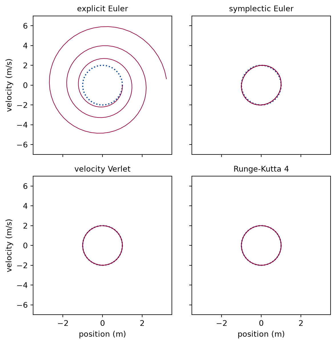
The angular frequency is $\omega$ = 2 rad/s, and the period is 3.142 s. Numerically verified (the oscillator at this step): Explicit Euler has multiplied the energy by 10.5 in three periods. The other three end close to the exact state. Velocity Verlet has the energy back to 6.1e-07 of the start although it did not conserve it along the way, and Runge-Kutta is 8.2 parts per million below the start, which is the drain the explanation derived. In phase space the difference is visible at a glance:

def draw_integrators_phase_space() -> Figure:
    """Three periods in phase space for each method, against the exact
    ellipse."""
    exact_orbit = harmonic_motion(released, mass, k, np.linspace(0.0, period, 200))

    fig, axes = plt.subplots(2, 2, figsize=(6.4, 6.4), sharex=True, sharey=True)
    for ax, integrator in zip(axes.flat, INTEGRATORS, strict=True):
        trajectory, _ = run_method(integrator, coarse, coarse_periods)
        ax.plot(
            exact_orbit.x[:, 0],
            exact_orbit.v[:, 0],
            color="#00429d",
            linestyle=":",
            label="exact",
        )
        ax.plot(trajectory.x[:, 0], trajectory.v[:, 0], color="#93003a", linewidth=0.8)
        ax.set_title(integrator.name, fontsize=10)
        ax.set_xlim(-3.5, 3.5)
        ax.set_ylim(-7.0, 7.0)
        ax.set_aspect(1 / omega)
    for ax in axes[1]:
        ax.set_xlabel("position (m)")
    for ax in axes[:, 0]:
        ax.set_ylabel("velocity (m/s)")
    fig.tight_layout()
    return fig

src/pbc/mechanics/experiments/numerical_integrators.py, lines 185 to 210, read from the repository when this page was built.

Figure 2: simulated Three periods in phase space for each method at the same coarse step, against the exact ellipse. Explicit Euler spirals outward and never returns; symplectic Euler stays on a closed curve that is tilted and wider than the ellipse; velocity Verlet and Runge-Kutta cannot be told from the ellipse at this scale.

The data are the runs of the table above, drawn against the exact ellipse of the oscillator; nothing in the picture is measured. The symplectic Euler curve does not spiral, and that is the first sign of the bounded energy that the long-run example quantifies.

Accuracy: the error against the step

The error of a run is the largest distance, over the whole run, between a simulated state and the exact one at the same time, measured in the plane of $x$ and $v/\omega$ so that position and velocity count alike. Dividing the velocity by $\omega$ turns it into the position it would reach in one radian of the oscillation, so the distance is in metres: a velocity error of $\omega$ metres per second counts as much as a position error of one metre. One instant would mislead: at a turning point a position error cannot show a phase error, and the first-order part of symplectic Euler’s error is periodic and vanishes at whole periods. The cell doubles the number of steps per period over two periods and tabulates the error and the observed order for each method.

def state_error(trajectory):
    """Largest distance from the exact state in the plane (x, v / omega), in m."""
    exact = harmonic_motion(released, mass, k, trajectory.t)
    dx = trajectory.x - exact.x
    dv = (trajectory.v - exact.v) / omega
    return np.max(np.sqrt(np.sum(dx**2 + dv**2, axis=1)))

src/pbc/mechanics/experiments/numerical_integrators.py, lines 213 to 218, read from the repository when this page was built.

step_counts = [25 * 2**i for i in range(6)]

src/pbc/mechanics/experiments/numerical_integrators.py, line 41, read from the repository when this page was built.

def error_orders(experiment: Experiment) -> dict:
    """The largest error over two periods for each method and step count,
    with the observed order; record the table and return the errors."""
    errors = {
        integrator.name: np.array(
            [state_error(run_method(integrator, n, 2)[0]) for n in step_counts]
        )
        for integrator in INTEGRATORS
    }

    columns = [("steps per period", "", "d")]
    for integrator in INTEGRATORS:
        columns += [(f"{integrator.name} error", "m", ".2e"), ("order", "", ".2f")]
    rows = []
    for i, n in enumerate(step_counts):
        row = [n]
        for integrator in INTEGRATORS:
            error = errors[integrator.name]
            row += [error[i], np.log2(error[i - 1] / error[i]) if i else None]
        rows.append(row)

    experiment.table(
        "error-orders",
        rows,
        columns=columns,
        caption="Largest error over two periods for each method, with the "
        "observed order from the previous row.",
    )
    return errors

src/pbc/mechanics/experiments/numerical_integrators.py, lines 221 to 249, read from the repository when this page was built.

Largest error over two periods for each method, with the observed order from the previous row.

steps per period	explicit Euler error (m)	order	symplectic Euler error (m)	order	velocity Verlet error (m)	order	Runge-Kutta 4 error (m)	order
25	3.67e+00		1.55e-01		3.54e-02		4.18e-04
50	1.19e+00	1.62	7.01e-02	1.15	8.83e-03	2.00	2.61e-05	4.00
100	4.83e-01	1.30	3.32e-02	1.08	2.21e-03	2.00	1.63e-06	4.00
200	2.18e-01	1.15	1.62e-02	1.04	5.51e-04	2.00	1.02e-07	4.00
400	1.04e-01	1.07	7.97e-03	1.02	1.38e-04	2.00	6.38e-09	4.00
800	5.06e-02	1.04	3.96e-03	1.01	3.45e-05	2.00	3.99e-10	4.00

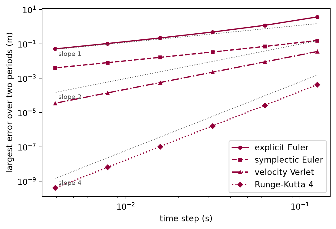
Numerically verified (the oscillator, two periods): The observed orders settle at the orders of the explanation: one, one, two, and four. The two first-order methods approach one from above, because at the coarser steps their errors contain the higher powers of $\omega\,\Delta t$ as well, and they do so from very different starting points: at the same step symplectic Euler is 24 times as accurate as explicit Euler at the coarsest step, at the same cost per step. On logarithmic axes the four errors are straight lines whose slopes are the orders:

def draw_integrators_convergence(errors: dict) -> Figure:
    """The largest error against the time step for the four methods."""
    steps = period / np.array(step_counts)
    styles = {
        "explicit Euler": ("o", "-"),
        "symplectic Euler": ("s", "--"),
        "velocity Verlet": ("^", "-."),
        "Runge-Kutta 4": ("D", ":"),
    }

    fig, ax = plt.subplots(figsize=(6.4, 4.2))
    for integrator in INTEGRATORS:
        marker, linestyle = styles[integrator.name]
        ax.loglog(
            steps,
            errors[integrator.name],
            color="#93003a",
            marker=marker,
            linestyle=linestyle,
            markersize=4,
            label=integrator.name,
        )
    for slope, anchor in ((1, 1.5), (2, 0.15), (4, 1.5e-3)):
        ax.loglog(
            steps,
            anchor * (steps / steps[0]) ** slope,
            color="#555555",
            linestyle=":",
            linewidth=0.8,
        )
        ax.annotate(
            f"slope {slope}",
            (steps[-1], anchor * (steps[-1] / steps[0]) ** slope),
            textcoords="offset points",
            xytext=(4, -8),
            fontsize=8,
            color="#555555",
        )
    ax.set_xlabel("time step (s)")
    ax.set_ylabel("largest error over two periods (m)")
    ax.legend(loc="lower right")
    return fig

src/pbc/mechanics/experiments/numerical_integrators.py, lines 252 to 293, read from the repository when this page was built.

Figure 3: simulated Largest error over two periods against the time step, for the four methods, with reference lines for the slopes one, two, and four. Each method follows the reference line of its order, so a tenfold smaller step buys one digit from explicit and symplectic Euler, two from velocity Verlet, and four from Runge-Kutta.

The errors come from the table above and the exact solution; the reference lines are drawn for comparison only. The straight lines say nothing about steps far finer than the ones plotted, where round-off takes over, or far coarser, where the stability limits of the explanation do.

Energy over a long run

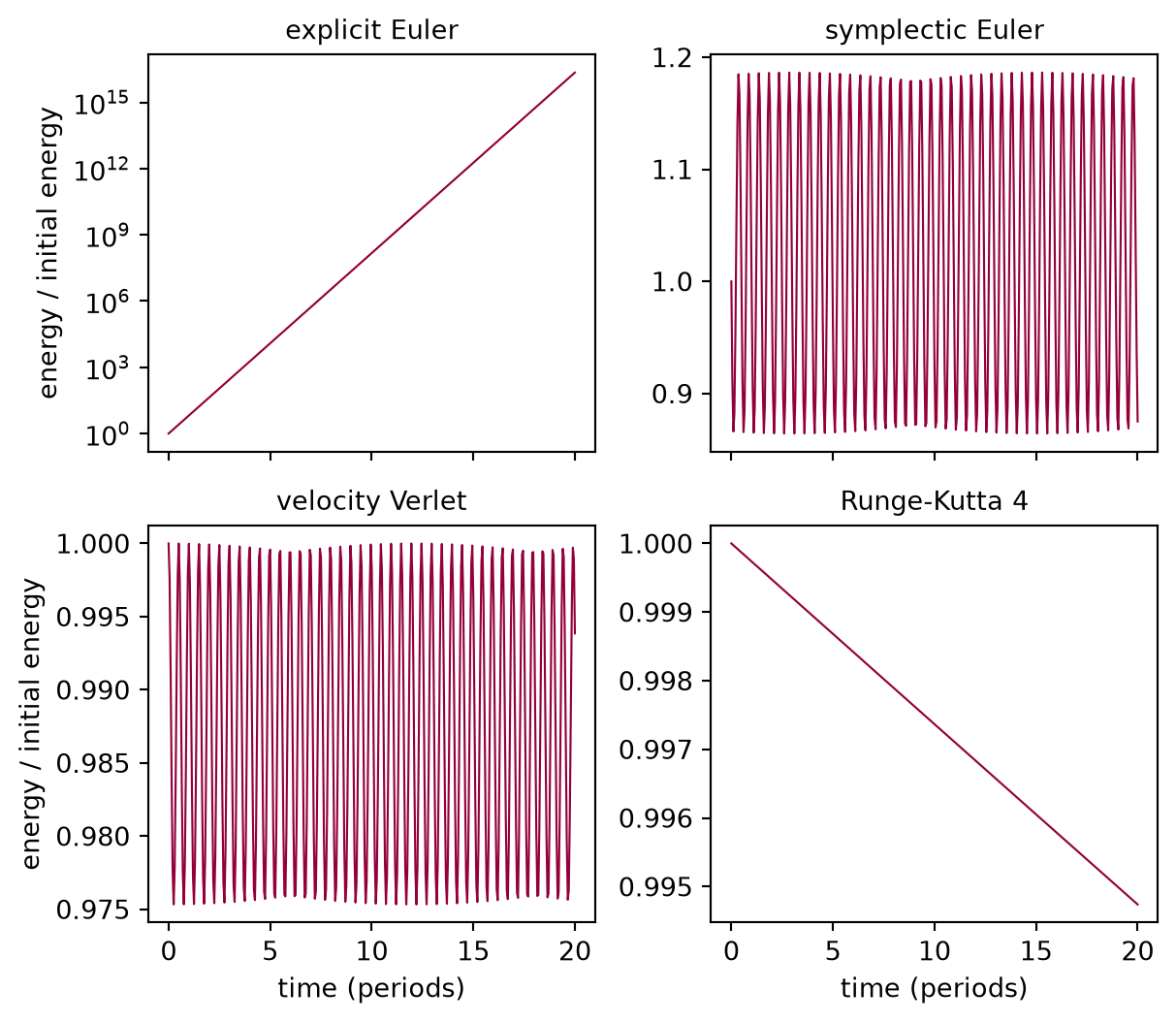
Twenty periods at twenty steps per period, $\omega\,\Delta t$ = 0.314, with the energy of every state relative to the initial energy. Each panel has its own vertical scale, because the four behaviours differ by many orders of magnitude.

n_periods, n = 20, 20
z = omega * period / n
dt = period / n
long_n, long_periods = 32, 1000

src/pbc/mechanics/experiments/numerical_integrators.py, lines 45 to 48, read from the repository when this page was built.

def draw_integrators_energy() -> Figure:
    """The energy over twenty periods at twenty steps per period."""
    fig, axes = plt.subplots(2, 2, figsize=(6.4, 5.6), sharex=True)
    for ax, integrator in zip(axes.flat, INTEGRATORS, strict=True):
        trajectory, _ = run_method(integrator, n, n_periods)
        relative = energy(trajectory, mass, k)
        ax.plot(
            trajectory.t / period,
            relative / relative[0],
            color="#93003a",
            linewidth=0.8,
        )
        if integrator.name == "explicit Euler":
            ax.set_yscale("log")
        ax.set_title(integrator.name, fontsize=10)
    for ax in axes[1]:
        ax.set_xlabel("time (periods)")
    for ax in axes[:, 0]:
        ax.set_ylabel("energy / initial energy")
    fig.tight_layout()
    return fig

src/pbc/mechanics/experiments/numerical_integrators.py, lines 296 to 316, read from the repository when this page was built.

Figure 4: simulated Energy relative to the initial energy over twenty periods at twenty steps per period; each panel has its own vertical scale. Explicit Euler gains energy at a constant rate, which is a straight line on the logarithmic axis. The two symplectic methods oscillate in a band that does not widen, narrower for velocity Verlet. Runge-Kutta loses energy slowly and steadily.

The next cell checks the four behaviours against the formulas of the explanation, on the same runs: the per-step factors for explicit Euler and Runge-Kutta, and the modified energies for the two symplectic methods.

def relative_energy(trajectory):
    e = energy(trajectory, mass, k)
    return e / e[0]

src/pbc/mechanics/experiments/numerical_integrators.py, lines 319 to 321, read from the repository when this page was built.

def ratios(trajectory):
    e = energy(trajectory, mass, k)
    return e[1:] / e[:-1]

src/pbc/mechanics/experiments/numerical_integrators.py, lines 324 to 326, read from the repository when this page was built.

def spread(values):
    """Largest relative deviation from the first value."""
    return np.max(np.abs(values / values[0] - 1))

src/pbc/mechanics/experiments/numerical_integrators.py, lines 329 to 331, read from the repository when this page was built.

def energy_formulas(experiment: Experiment):
    """The energy formulas of the explanation against the runs of the
    figure; record the table and return the runs and modified energies."""
    results = {
        integrator.name: run_method(integrator, n, n_periods)[0]
        for integrator in INTEGRATORS
    }
    euler, symplectic, verlet, rk4 = (results[i.name] for i in INTEGRATORS)
    modified_se = (
        0.5
        * mass
        * (
            symplectic.v[:, 0] ** 2
            + omega**2 * symplectic.x[:, 0] ** 2
            - omega**2 * dt * symplectic.x[:, 0] * symplectic.v[:, 0]
        )
    )
    modified_vv = (
        0.5
        * mass
        * (
            verlet.v[:, 0] ** 2
            + omega**2 * (1 - omega**2 * dt**2 / 4) * verlet.x[:, 0] ** 2
        )
    )
    rk4_factor = 1 - z**6 / 72 + z**8 / 576

    experiment.table(
        "energy-formulas",
        [
            (
                "explicit Euler",
                "ratio per step",
                ratios(euler)[0],
                1 + z**2,
                np.max(np.abs(ratios(euler) - (1 + z**2))),
            ),
            (
                "Runge-Kutta 4",
                "ratio per step",
                ratios(rk4)[0],
                rk4_factor,
                np.max(np.abs(ratios(rk4) - rk4_factor)),
            ),
            ("symplectic Euler", "modified energy", None, None, spread(modified_se)),
            ("velocity Verlet", "modified energy", None, None, spread(modified_vv)),
        ],
        columns=[
            ("method", "", ""),
            ("quantity", "", ""),
            ("computed", "", ".8f"),
            ("derived", "", ".8f"),
            ("largest deviation", "", ".1e"),
        ],
        caption="The energy formulas of the explanation against the runs of the "
        "figure: the per-step energy ratio, and how far the modified energy "
        "strays from constant.",
    )
    return symplectic, verlet, modified_se, modified_vv, rk4_factor

src/pbc/mechanics/experiments/numerical_integrators.py, lines 334 to 392, read from the repository when this page was built.

The energy formulas of the explanation against the runs of the figure: the per-step energy ratio, and how far the modified energy strays from constant.

method	quantity	computed	derived	largest deviation
explicit Euler	ratio per step	1.09869604	1.09869604	4.4e-16
Runge-Kutta 4	ratio per step	0.99998681	0.99998681	3.3e-16
symplectic Euler	modified energy			1.0e-15
velocity Verlet	modified energy			4.0e-15

Every formula holds to round-off. The two symplectic methods conserve their modified energies to about 4e-15, which is why the true energy oscillates within a fixed band in the figure and never leaves it. The true energy of symplectic Euler stays between 0.8642 and 1.1863 times the start, a band as wide as $\omega\,\Delta t$ = 0.31; velocity Verlet stays between 0.9753 and 1.0000, a band of about $\omega^2 \Delta t^2 / 4$ = 0.025. Runge-Kutta loses 13.2 parts per million per step, a steady drain that no refinement of the digits of the step changes in sign. Over a thousand periods the difference between bounded and steady shows plainly. The cell runs the three methods that can be run that far at 32 steps per period and tabulates the energy and, for the reader who would trust the position as well, the largest state error; explicit Euler would multiply the energy by ten to the power 525 and is left out.

def long_run_energy_bands(experiment: Experiment):
    """A thousand periods at thirty-two steps per period for the methods
    after explicit Euler; record the table and return the largest state
    error and the lowest energy of each."""
    long_runs, long_lowest = {}, {}
    rows = []
    for integrator in INTEGRATORS[1:]:
        trajectory, calls = run_method(integrator, long_n, long_periods)
        relative = relative_energy(trajectory)
        long_runs[integrator.name] = state_error(trajectory)
        long_lowest[integrator.name] = np.min(relative)
        rows.append(
            (
                integrator.name,
                np.min(relative),
                np.max(relative),
                relative[-1],
                long_runs[integrator.name],
                calls,
            )
        )

    experiment.table(
        "long-run-energy-bands",
        rows,
        columns=[
            ("method", "", ""),
            ("lowest energy / initial", "", ".5f"),
            ("highest energy / initial", "", ".5f"),
            ("energy / initial at the end", "", ".5f"),
            ("largest state error", "m", ".3f"),
            ("calls", "", "d"),
        ],
        caption="A thousand periods at thirty-two steps per period: the range of "
        "the energy, and the largest distance from the exact state.",
    )
    return long_runs, long_lowest

src/pbc/mechanics/experiments/numerical_integrators.py, lines 395 to 431, read from the repository when this page was built.

A thousand periods at thirty-two steps per period: the range of the energy, and the largest distance from the exact state.

method	lowest energy / initial	highest energy / initial	energy / initial at the end	largest state error (m)	calls
symplectic Euler	0.91060	1.10886	0.91071	2.053	32000
velocity Verlet	0.99036	1.00000	0.99588	2.000	64000
Runge-Kutta 4	0.97497	1.00000	0.97497	0.077	128000

Numerically verified (the oscillator at this step): The symplectic methods are still within their bands, which are no wider after a thousand periods than after one. Runge-Kutta has lost a measurable fraction of the energy and keeps losing it at the same rate. For a run that is long compared with the period, it is the symplectic methods that can be trusted with the energy, and velocity Verlet is the one with a narrow band. The last column is a warning: a bounded energy does not mean an accurate state, because a method can stay on a slightly wrong ellipse and traverse it at a slightly wrong rate, so that it ends in the wrong place of its orbit. For the position after a few periods it is Runge-Kutta, and the cost example says by how much.

Cost: a millimetre after two periods

How many calls to the acceleration does each method need to keep the error below one millimetre over two periods? The order answers it without a search. If the error at the finest step of the accuracy table is $\varepsilon$ and the method has order $p$, the step for the tolerance $\varepsilon_0$ is the finest step times $(\varepsilon_0/\varepsilon)^{1/p}$. The cell predicts the steps per period that way, runs each method at that step, and counts the calls.

def calls_for_one_millimetre(experiment: Experiment, errors: dict) -> dict:
    """The steps each method needs for an error of one millimetre over two
    periods, predicted from its order; record the table and return the
    calls of each."""
    tolerance = 1e-3  # m

    cost = {}
    rows = []
    for integrator in INTEGRATORS:
        finest_error = errors[integrator.name][-1]
        needed = int(
            np.ceil(
                step_counts[-1] * (finest_error / tolerance) ** (1 / integrator.order)
            )
        )
        trajectory, calls = run_method(integrator, needed, 2)
        cost[integrator.name] = calls
        rows.append((integrator.name, needed, state_error(trajectory), calls))

    experiment.table(
        "calls-for-one-millimetre",
        rows,
        columns=[
            ("method", "", ""),
            ("steps per period", "", "d"),
            ("error", "m", ".1e"),
            ("calls over two periods", "", "d"),
        ],
        caption="Steps predicted from the order for an error of one millimetre "
        "over two periods, with the error reached and the calls it took.",
    )
    return cost

src/pbc/mechanics/experiments/numerical_integrators.py, lines 434 to 465, read from the repository when this page was built.

Steps predicted from the order for an error of one millimetre over two periods, with the error reached and the calls it took.

method	steps per period	error (m)	calls over two periods
explicit Euler	40469	9.8e-04	80938
symplectic Euler	3165	9.9e-04	6330
velocity Verlet	149	9.9e-04	596
Runge-Kutta 4	21	8.4e-04	168

Every prediction lands just inside the tolerance, which is the order doing what it says. Numerically verified (the oscillator, tolerance of one millimetre): For one millimetre over two periods, Runge-Kutta needs 168 calls, velocity Verlet 596, symplectic Euler 6330, and explicit Euler 80938. The ratios only grow for a tighter tolerance: for one more digit explicit Euler needs ten times the calls and Runge-Kutta fewer than twice.

The rule that follows, for the rest of the course: for an accurate state over a short run, use Runge-Kutta; for the energy over a long run, use velocity Verlet; never use explicit Euler for an oscillation. Symplectic Euler is the method to understand, not to use: it shows that the order of the updates, not the number of evaluations, is what decides whether the energy is bounded.

Interactive visualization

The figures above fix the step. Here the step and the method are yours. The figure below shows the oscillator of this lesson, released at rest, for five periods, with all four methods at the same number of steps per period and the exact motion for comparison. With scripts enabled, choose the integrator to emphasise and to read out, and change the number of steps per period to see every curve respond. The interesting settings are the coarse ones: at four steps per period $\omega\,\Delta t$ is about 1.6, and the stability limits of the explanation decide which curves survive.

The runs behind the figure come from the cell below, which calls the tested integrators of this lesson for every method at nine step counts when the page is built. The script of the figure draws these results and computes no physics of its own.

    explorer = explorer_data(mass=mass, k=k)
    experiment.widget("integrator-explorer", explorer)

src/pbc/mechanics/experiments/numerical_integrators.py, lines 699 to 700, read from the repository when this page was built.

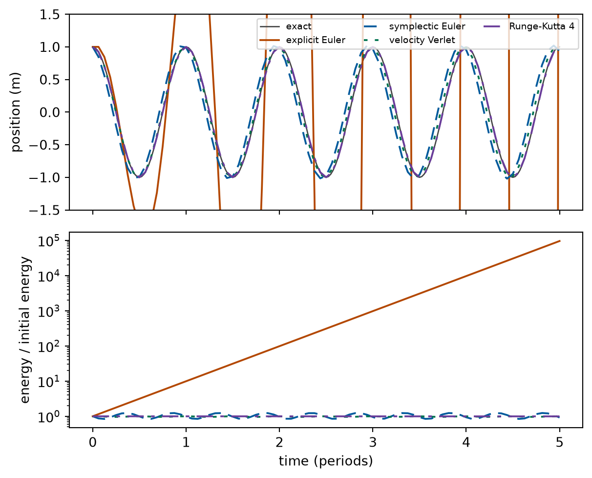
Figure 5: simulated Position and energy over five periods at a moderate step, for the four methods. The energy shows explicit Euler climbing while the others stay near the start. With scripts, the figure responds to the controls below it.

With JavaScript, this figure gets controls for the integrator and the number of steps per period. Without it, the figure above and the tables below show the results at the default step count (16 steps per period) and at every other step count.

Whatever the script can show is also in these tables: for each step count the figure offers, the energy after five periods relative to the start, the largest position error over the run, and the number of evaluations of the acceleration, for each method.

Energy after five periods relative to the initial energy, for each step count of the figure.

steps per period	explicit Euler	symplectic Euler	velocity Verlet	Runge-Kutta 4
4	6.311e+10	4.233	0.3832	0.04432
6	4.422e+09	1.846	0.7275	0.6201
8	2.222e+08	0.7917	0.91	0.8865
12	2.058e+06	0.8362	0.991	0.9836
16	9.613e+04	0.9234	0.9984	0.996
24	2850	0.9765	0.9999	0.9995
32	425.2	0.9901	1	0.9999
50	50.25	0.9974	1	1
100	7.171	0.9997	1	1

Largest position error over five periods, for each step count of the figure.

steps per period	explicit Euler (m)	symplectic Euler (m)	velocity Verlet (m)	Runge-Kutta 4 (m)
4	1.32e+05	2.60e+00	1.99e+00	8.09e-01
6	4.24e+04	1.69e+00	1.35e+00	2.44e-01
8	9.09e+03	1.15e+00	7.35e-01	9.34e-02
12	1.25e+03	5.99e-01	3.45e-01	1.88e-02
16	2.30e+02	3.90e-01	1.94e-01	5.97e-03
24	4.02e+01	2.17e-01	8.58e-02	1.18e-03
32	1.80e+01	1.47e-01	4.81e-02	3.72e-04
50	5.99e+00	8.25e-02	1.97e-02	6.22e-05
100	1.68e+00	3.63e-02	4.91e-03	3.88e-06

Evaluations of the acceleration over five periods, for each step count of the figure.

steps per period	explicit Euler	symplectic Euler	velocity Verlet	Runge-Kutta 4
4	20	20	40	80
6	30	30	60	120
8	40	40	80	160
12	60	60	120	240
16	80	80	160	320
24	120	120	240	480
32	160	160	320	640
50	250	250	500	1000
100	500	500	1000	2000

Limits

What this lesson shows is a statement about four fixed-step methods on one linear system and one drag example, not about numerical integration in general.

• The formulas for the energy per step, the matrices, and the modified energies are exact for the linear oscillator only. For a nonlinear force the lesson makes no claim about the energy: the bounded band of the symplectic methods and the steady drift of the others are results for the oscillator, not general properties, and are not demonstrated here; the next lesson looks at a pendulum.
• The bands of the energy are shown at the steps of the figures. That they narrow with the step, as the modified energies say, is derived here and confirmed by the conserved quantities to round-off, but not plotted against the step.
• With a force that depends on the velocity, only the orders are measured (second exercise). Nothing here says that the predicted-velocity version of velocity Verlet keeps the reversibility or the long-run behaviour of its position-only form.
• Cost is counted in evaluations of the force. A real force may be cheap enough that the arithmetic around it matters, or costly enough that carrying the acceleration over, which saves one call per step for velocity Verlet, decides the choice.
• A step that is not fixed is not covered. Methods that estimate their own error and choose the step, such as the adaptive pair behind RK45 of SciPy, are the standard tool for a trajectory with fast and slow parts; their order, cost, and energy behaviour differ from the classical method of this lesson.
• Round-off is stated as negligible, and the finest step of the accuracy table stays far above it; the lesson never reaches the step at which it would matter.

Self-check. Velocity Verlet at thirty-two steps per period keeps the energy of the oscillator inside a narrow band for a thousand periods. Does it follow that its position after a thousand periods is as accurate as after two? Say what the table of the long run shows, and why.

With scripts, you can record in this browser that you answered this question.

Solution to the self-check

No. The energy says only that the state lies on a closed curve close to the true one; it says nothing about where on the curve the state is. The method turns the state by an angle per step that is slightly wrong, so the phase error grows with time while the energy stays bounded. The long-run table shows it: the largest state error of velocity Verlet over the thousand periods is 2.00 m, the whole width of the orbit of amplitude one metre, so at some time the state was on the far side of the orbit from the exact one, although its energy is within 1.0 per cent of the start. The first assumption that fails is the one about what “accurate” means: bounded energy error and small position error are different properties, and the first does not imply the second.

Exercises

Exercise 1. At the limit. Predict what each method does at 3.5, 3, and 2.2 steps per period, from the stability limits of the explanation, then run 100 steps with each and print the energy relative to the start.

Hint 1 of 2 for exercise 1

Turn a number of steps per period into the product of the angular frequency and the time step. The stability limits of the explanation are stated for that product.

Hint 2 of 2 for exercise 1

Compare that product with the limit of each method. A method whose product is above its limit grows without bound; one below it does not.

Solution to exercise 1

Symplectic Euler and velocity Verlet are stable below $z = 2$, so they survive the first step size and blow up at the other two. The classical Runge-Kutta method is stable below $z = 2\sqrt 2$, so it survives the first two and blows up at the third. Explicit Euler grows at all three, by the factor $1 + \omega^2 \Delta t^2$ per step.

def stability_limits(experiment: Experiment) -> None:
    """Exercise 1: the energy after one hundred steps near the stability
    limits; record the table."""
    rows = []
    for steps_per_period in (3.5, 3.0, 2.2):
        row = [steps_per_period, 2 * np.pi / steps_per_period]
        for integrator in INTEGRATORS:
            trajectory = simulate(
                released,
                oscillator,
                period / steps_per_period,
                100,
                step=integrator.step,
            )
            row.append(relative_energy(trajectory)[-1])
        rows.append(row)

    experiment.table(
        "stability-limits",
        rows,
        columns=[("steps per period", "", ".1f"), ("omega dt", "", ".3f")]
        + [(f"{i.name}, energy / initial", "", ".2e") for i in INTEGRATORS],
        caption="Energy relative to the start after one hundred steps, at three "
        "steps near the stability limits.",
    )

src/pbc/mechanics/experiments/numerical_integrators.py, lines 541 to 565, read from the repository when this page was built.

Energy relative to the start after one hundred steps, at three steps near the stability limits.

steps per period	omega dt	explicit Euler, energy / initial	symplectic Euler, energy / initial	velocity Verlet, energy / initial	Runge-Kutta 4, energy / initial
3.5	1.795	3.63e+62	2.09e+00	9.70e-01	7.54e-15
3.0	2.094	1.35e+73	1.08e+54	4.01e+52	1.81e-33
2.2	2.856	1.49e+96	5.10e+155	1.55e+155	9.56e+05

At the first step size the two symplectic methods are stable and their energy is still within a band, though a wide one so close to the limit. Runge-Kutta at that step has lost nearly all the energy: its factor per step is far below one there, so “stable” means only that nothing grows. A method near its stability limit is not accurate; it is merely not exploding.

Exercise 2. A force that depends on the velocity. The Newton’s laws lesson has an exact solution for a throw with linear drag. Do velocity Verlet and Runge-Kutta 4 keep their orders when the force depends on the velocity? Measure them on that throw, over the first two seconds, against the exact solution.

Hint 1 of 2 for exercise 2

The error of one run is the distance between the simulated and the exact position at the end. Which module of the Newton’s laws lesson gives the exact solution?

Hint 2 of 2 for exercise 2

Halve the time step several times. The order is the base-two logarithm of the ratio of two successive errors.

Solution to exercise 2

The drag force and the exact solution come from pbc.mechanics.drag; the error is the distance between the simulated and the exact position after two seconds.

def throw_with_drag(experiment: Experiment) -> None:
    """Exercise 2: the position error of a throw with linear drag after two
    seconds, for velocity Verlet and Runge-Kutta; record the table."""
    drag_mass, b = 0.5, 0.25  # kg, kg/s: time constant 2 s
    thrown = State(t=0.0, x=[0.0, 0.0], v=[12.0, 15.0])
    with_drag = newton(drag_mass, weight(drag_mass, [0.0, -g]), linear_drag(b))
    duration = 2.0  # s
    exact_throw = fall_with_linear_drag(thrown, drag_mass, b, [0.0, -g], duration)

    previous = {}
    rows = []
    for n_steps in (20, 40, 80, 160, 320):
        row = [n_steps]
        for integrator in INTEGRATORS[2:]:
            trajectory = simulate(
                thrown, with_drag, duration / n_steps, n_steps, step=integrator.step
            )
            error = np.linalg.norm(trajectory.x[-1] - exact_throw.x[0])
            order = (
                np.log2(previous[integrator.name] / error)
                if integrator.name in previous
                else None
            )
            previous[integrator.name] = error
            row += [error, order]
        rows.append(row)

    experiment.table(
        "throw-with-drag",
        rows,
        columns=[("steps", "", "d")]
        + [
            column
            for integrator in INTEGRATORS[2:]
            for column in (
                (f"{integrator.name} error", "m", ".2e"),
                ("order", "", ".2f"),
            )
        ],
        caption="Position error after two seconds of a throw with linear drag, "
        "with the observed order.",
    )

src/pbc/mechanics/experiments/numerical_integrators.py, lines 568 to 609, read from the repository when this page was built.

Position error after two seconds of a throw with linear drag, with the observed order.

steps	velocity Verlet error (m)	order	Runge-Kutta 4 error (m)	order
20	1.17e-02		1.46e-06
40	2.86e-03	2.03	8.96e-08	4.03
80	7.09e-04	2.01	5.54e-09	4.02
160	1.76e-04	2.01	3.45e-10	4.01
320	4.40e-05	2.00	2.15e-11	4.00

Both keep their orders. For velocity Verlet that is what the predicted velocity in the second acceleration call is for; without it the method would fall to first order on any velocity-dependent force. What is lost with drag is not the order but the meaning of “symplectic”: there is no conserved energy for the method to shadow.

Exercise 3. Equal cost. Give each method 200 calls to the acceleration per period: 200 steps for the two Euler methods, 100 for velocity Verlet, 50 for Runge-Kutta 4. Which has the smallest error over two periods, and by how much?

Hint 1 of 2 for exercise 3

The cost is the number of calls to the acceleration. How many calls does one step of each method make?

Hint 2 of 2 for exercise 3

Divide the budget of calls by the calls per step to get the steps per period of each method, then compare the largest errors.

Solution to exercise 3

def equal_cost(experiment: Experiment) -> dict:
    """Exercise 3: the largest error over two periods when every method has
    two hundred calls per period; record the table."""
    budget = 200  # calls per period
    equal_cost = {}
    rows = []
    for integrator in INTEGRATORS:
        steps_per_period = budget // integrator.evaluations
        trajectory, calls = run_method(integrator, steps_per_period, 2)
        equal_cost[integrator.name] = state_error(trajectory)
        rows.append(
            (integrator.name, steps_per_period, calls, equal_cost[integrator.name])
        )

    experiment.table(
        "equal-cost",
        rows,
        columns=[
            ("method", "", ""),
            ("steps per period", "", "d"),
            ("calls", "", "d"),
            ("largest error", "m", ".1e"),
        ],
        caption="Largest error over two periods when every method has the same "
        "number of calls per period.",
    )
    return equal_cost

src/pbc/mechanics/experiments/numerical_integrators.py, lines 612 to 638, read from the repository when this page was built.

Largest error over two periods when every method has the same number of calls per period.

method	steps per period	calls	largest error (m)
explicit Euler	200	400	2.2e-01
symplectic Euler	200	400	1.6e-02
velocity Verlet	100	400	2.2e-03
Runge-Kutta 4	50	400	2.6e-05

At equal cost the ranking is the ranking by order, and the gaps are large: velocity Verlet is 7 times as accurate as symplectic Euler although it takes half the steps, and Runge-Kutta is 84 times as accurate as velocity Verlet with half of those. The one case in which a lower order wins at equal cost is a run long enough for Runge-Kutta’s energy drain to matter, which is the long-run example.

Run this experiment

This page was built from commit 6417e2ff90258bd2d2ba21d217eb7666fd24f680 of the repository.

In a clone at that commit, with the project’s Python packages installed, this command runs the experiment of this page:

uv run --locked --no-dev python -m pbc.mechanics.experiments.numerical_integrators results

Files, tests, and every command

The files behind it:

• site/lessons/mechanics/05-numerical-integrators/index.qmd: this page, with every code cell.
• src/pbc/mechanics/dynamics.py: code the experiment runs.
• src/pbc/mechanics/integrators.py: code the experiment runs.
• src/pbc/mechanics/oscillator.py: code the experiment runs.
• src/pbc/mechanics/drag.py: code the experiment runs.
• src/pbc/mechanics/explorer.py: code the experiment runs.
• src/pbc/mechanics/experiments/numerical_integrators.py: code the experiment runs.
• src/pbc/experiment.py: code the experiment runs.
• src/pbc/authoring/widgets.py: code the experiment runs.
• site/widgets/integrator-explorer.js: code the experiment runs.
• tests/unit/test_dynamics.py: tests of that code.
• tests/unit/test_integrators.py: tests of that code.
• tests/unit/test_oscillator.py: tests of that code.
• tests/unit/test_drag.py: tests of that code.
• tests/unit/test_explorer.py: tests of that code.
• tests/unit/test_widgets.py: tests of that code.
• tests/unit/test_numerical_integrators_experiment.py: tests of that code.

With Git and uv installed (see the setup page), run:

git clone https://github.com/taspinar/physics-by-construction.git
cd physics-by-construction
git checkout 6417e2ff90258bd2d2ba21d217eb7666fd24f680
uv sync --locked --no-dev
uv run --locked --no-dev python -m pbc.mechanics.experiments.numerical_integrators results

The experiment writes every figure of this page into results/, as <label>.png, and every number and table of the page, as the page shows it, into results/results.json. Its numbers match this page to the digits shown, and its figure files are the ones the page shows; digits beyond those can differ between machines, because floating-point libraries differ. Change the code of the experiment and run it again to see what changes.