Automated analysis pipelines

One reusable workflow, a parameter sweep, a statistic with its uncertainty, a figure, and a report that the build regenerates and compares with a committed expectation, run on a simulated throw and on measured waves.

Course

Classical mechanics, lesson 23 of 28

Slot

R1, number 1 of the 6 slots of the path Autonomous scientific research

Methods

Simulation, Measured data

Difficulty

Intermediate, level 2 of 3

What you’ll learn

Write an analysis as a function that a sweep, a repetition, and a report can all reuse
Carry the uncertainty of an input to a result, and check that propagation with a seeded Monte Carlo run
Tell the scatter of repetitions from the effect of an analysis choice, and report both
Turn the numbers of an analysis into a report that a build compares with a committed expectation

Prerequisites

Projectile motion with quadratic drag.

Before you begin

Statistics: the mean, the standard deviation, and the standard error of a mean

Related

none

Previous

Verifying scientific code

Next

Gravitational-wave strain lab

With scripts, this page keeps a record in your browser of whether you completed the lesson. Nothing is stored without them.

With scripts, this place suggests what to do next, with the reason, from the progress saved in your browser. Without them, follow the learning path.

A result that someone computed by hand once, and pasted into a document, cannot be trusted a second time. Nobody can say which inputs it came from, which choices went into it, or whether it still holds after the code changed. The physical question of this lesson is how to make an analysis that answers the same way every time it is asked, and that says so when it does not.

The answer has four parts, and the lesson builds each on two problems. An analysis is a function, so that a sweep can call it for many values of a parameter. Its result carries an uncertainty, which comes from the inputs and from the choices of the analysis. Its numbers are collected in a report, and the report is shown at the precision a reader sees. The build then regenerates the report and compares it with a committed expectation: when a number a reader would see changes, the build fails and says which line.

The first problem is simulated: how far a ball goes when the launch speed is only known to a standard uncertainty, as a function of the launch angle. The second is measured: the height and the period of waves over a submerged bar in a wave flume, from five repetitions of one experiment. They are two problems with one workflow, and the second one shows what the first cannot: the scatter between repetitions is small, and the choice of the window of the analysis is not.

Assumptions

The function is deterministic. The same inputs give the same numbers, so a report can be compared with an expectation. A function that draws random numbers takes a seed; without one, no expectation can hold.
Uncertainties are independent and small. The propagation is first order: it replaces the function by its tangent at the input. For a large relative uncertainty, or inputs that share an error, it is wrong, and the Monte Carlo run is the check.
Repetitions are independent. The standard error of the mean falls with the square root of their number only when the repetitions do not share an error. The five records of the flume were aligned on another gauge; a shared error of that alignment is not in their scatter.
The report is compared as it is shown. Two reports agree when their text agrees, so a change below the displayed precision passes, and a change in the last shown digit fails. A value that sits at a rounding boundary can flip on another machine; the precision is chosen well above round-off to avoid that.
An expectation is a record, not a proof. It says the analysis gives the numbers it gave when someone last accepted them. Whether they are right comes from the tests of the earlier lessons and from the checks below.

What the workflow does

An analysis starts as a function $f(\theta)$ of one parameter $\theta$ and returns the quantities one wants. A sweep evaluates it on a list of values and keeps the results in a table: the launch angle against the range, the end of a window against the wave height. The sweep is how a reader sees how much a result depends on a choice.

Uncertainty of an input. A launch speed $v$ known to a standard uncertainty $\sigma_v$ gives a range $R(v)$ with the uncertainty $\sigma_R \approx \left|\frac{\mathrm{d}R}{\mathrm{d}v}\right|\,\sigma_v ,$ the tangent of $R$ at the input times its uncertainty. The derivative has no formula once drag is in, so it is a central difference of the simulation itself, which is what pbc.data.uncertainty.propagate does. A Monte Carlo run checks it without the tangent: draw many speeds from a normal distribution with the standard deviation $\sigma_v$ , compute the range of each, and compare the spread of the ranges with $\sigma_R$ .

Repetitions. Of $n$ independent repetitions of a measurement, the mean is the best value and its standard uncertainty is the standard error, $\sigma_{\bar{x}} = \frac{s}{\sqrt{n}},$ with $s$ the standard deviation of the repetitions. This number says how far the mean would move on a new set of repetitions. It says nothing about a choice of the analysis, for example which seconds of the record count as the steady wave train. A result is honest when both are reported: the standard error, and how much the result moves when the choice is varied within what is reasonable.

The report. The quantities are listed in a fixed order, each with its unit, its uncertainty if it has one, and the number of decimals it is shown with. The report is the text a reader sees, one line per quantity. The expectation is the same text, committed. The comparison is exact on the text, which is the same as comparing the numbers at the displayed precision.

The program

The helpers are in pbc.data.pipeline, and the two problems use them. The listings are read from the files when the site is built.

def sweep(
    parameter: str,
    values: Sequence[float],
    func: Callable[[float], Mapping[str, float]],
    *,
    unit: str = "",
) -> Sweep:
    """Evaluate ``func`` at each of ``values``; ``func`` returns named results.

    Every call has to return the same names, so that the sweep is a table.
    """
    grid = np.asarray(values, dtype=float)
    if grid.ndim != 1 or grid.size == 0:
        raise ValueError("a sweep needs a one-dimensional, non-empty list of values")
    answers = [dict(func(float(v))) for v in grid]
    names = tuple(answers[0])
    for answer in answers:
        if set(answer) != set(names):
            raise ValueError(
                "the function returned different results for different values"
            )
    results = {n: np.array([a[n] for a in answers], dtype=float) for n in names}
    return Sweep(parameter, unit, grid, results)

src/pbc/data/pipeline.py, lines 48 to 70, read from the repository when this page was built.

A sweep calls the function once per value and insists that every call returns the same names, so the result is a table and not a list of dictionaries that might differ. The report and its comparison:

def differences(report: Report, expected: str) -> list[str]:
    """What differs between the report as shown and the ``expected`` text.

    One message per line that is changed, missing, or new. Empty when a reader
    sees the same report.
    """
    shown = report.render().splitlines()
    wanted = expected.splitlines()
    out = []
    for k in range(max(len(shown), len(wanted))):
        got = shown[k] if k < len(shown) else None
        want = wanted[k] if k < len(wanted) else None
        if got != want:
            out.append(f"line {k + 1}: expected {want!r}, the build produced {got!r}")
    return out

src/pbc/data/pipeline.py, lines 153 to 167, read from the repository when this page was built.

differences compares the report as shown with the expectation, line by line, and names each line that changed, is missing, or is new. check_report raises ReportMismatch with those messages, which is what fails the build. The expectation is updated on purpose, with python -m pbc.data.reports --update, and the change is read in the diff of the commit.

Worked examples

A simulated throw: the angle sweep

A baseball is thrown at a speed of 30 m/s with a standard uncertainty of 0.5 m/s, in air at sea level. The function that the whole pipeline reuses is the range of one throw. The step is fixed and the stepper is the classical fourth-order method, so the integration error is far below the uncertainties that follow.

def range_with_uncertainty(angle: float) -> dict[str, float]:
    """Range at ``angle`` with the uncertainty that the speed's one carries into it.

    First order and independent inputs: ``sigma_range = |d range / d speed| *
    sigma_speed`` by ``pbc.data.uncertainty.propagate``.
    """
    value, sigma = propagate(
        lambda speed: np.array(throw_range(float(speed), angle)),
        [SPEED],
        [SPEED_SIGMA],
    )
    return {
        "range": float(value),
        "sigma": float(sigma),
        "no_drag": float(drag_free_range(SPEED, angle)),
    }

src/pbc/mechanics/analysis.py, lines 41 to 56, read from the repository when this page was built.

The sweep calls it for seven angles. The table has the range, the uncertainty that the speed carries into it, and the range the same throw would have without drag, which is the closed form of the earlier lessons.

def angle_sweep():
    """The range for each launch angle with its uncertainty; the sweep, the
    share lost to drag, and the relative uncertainty, in per cent."""
    scan = analysis.angle_sweep()
    loss = 100 * (1 - scan.results["range"] / scan.results["no_drag"])
    relative = 100 * scan.results["sigma"] / scan.results["range"]
    return scan, loss, relative

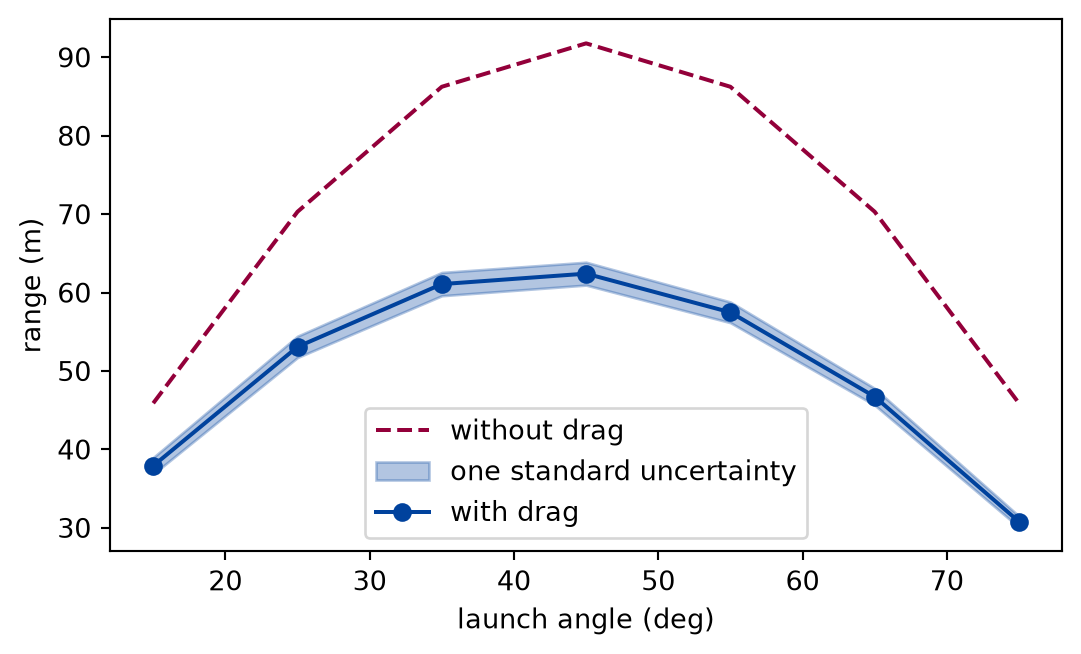
src/pbc/mechanics/experiments/automated_analysis_pipelines.py, lines 29 to 35, read from the repository when this page was built.

The range with drag is below the drag-free range at every angle, by 17 to 34 per cent of it, and the uncertainty is 2.3 to 2.8 per cent of the range. The maximum of the coarse grid is at 45 degrees. A finer sweep around it finds the angle that gives the longest throw:

def fine_sweep():
    """The best angle on the fine grid around the maximum, in degrees."""
    fine = analysis.fine_sweep()
    best = fine.argmax("range")
    print(f"best angle on the fine grid: {best:.1f} degrees")
    return best

src/pbc/mechanics/experiments/automated_analysis_pipelines.py, lines 38 to 43, read from the repository when this page was built.

best angle on the fine grid: 42.5 degrees

Numerically verified (this ball, speed, and air): Drag moves the angle of the longest throw below the drag-free value of forty-five degrees, to 42.5 degrees on the grid. The sweep finds the effect without a formula; why drag moves the angle is the subject of the earlier lesson on drag.

def draw_range_sweep(scan) -> Figure:
    """The range against the launch angle with its uncertainty band."""
    angles = scan.values
    range_fig, range_ax = plt.subplots(figsize=(6.4, 3.6))
    range_ax.plot(
        angles,
        scan.results["no_drag"],
        color=FIGURE_COLOURS[1],
        linestyle="--",
        label="without drag",
    )
    range_ax.fill_between(
        angles,
        scan.results["range"] - scan.results["sigma"],
        scan.results["range"] + scan.results["sigma"],
        color=FIGURE_COLOURS[0],
        alpha=0.3,
        label="one standard uncertainty",
    )
    range_ax.plot(
        angles,
        scan.results["range"],
        color=FIGURE_COLOURS[0],
        marker="o",
        label="with drag",
    )
    range_ax.set_xlabel("launch angle (deg)")
    range_ax.set_ylabel("range (m)")
    range_ax.legend()
    return range_fig

src/pbc/mechanics/experiments/automated_analysis_pipelines.py, lines 46 to 75, read from the repository when this page was built.

Line plot of range in metres against launch angle in degrees. A dashed curve for the throw without drag rises to a maximum at forty-five degrees and falls symmetrically. A solid curve for the throw with drag lies below it, with a maximum at a smaller angle. A shaded band about the solid curve shows one standard uncertainty, a little more than a metre wide on each side. — Figure 1: simulated Range of the throw against launch angle. With drag the range is lower and its maximum lies at a smaller angle than without; the band is one standard uncertainty from the launch speed.

The figure puts the sweep, the uncertainty, and the limiting case on one panel. It was drawn from the table above, and the drag-free curve is the closed form that the earlier lesson checked the simulation against.

The first-order uncertainty assumes that the range is a straight line in the speed over the width of $\sigma_v$ . The Monte Carlo run does not: it draws 200 speeds with a fixed seed, throws each, and takes the spread of the ranges.

def monte_carlo_check(experiment: Experiment, best):
    """The propagated uncertainty of the range at the best angle against the
    spread of a seeded Monte Carlo run; record the table."""
    _, spread = analysis.monte_carlo(best)
    propagated = analysis.range_with_uncertainty(best)["sigma"]
    experiment.table(
        "monte-carlo-check",
        [(propagated, spread, 100 * (spread / propagated - 1))],
        columns=[
            ("propagated uncertainty", "m", ".2f"),
            ("Monte Carlo spread", "m", ".2f"),
            ("difference", "%", ".0f"),
        ],
        caption="The first-order uncertainty of the range at the best angle and "
        "the spread of a seeded Monte Carlo run, to two decimals.",
    )
    return propagated, spread

src/pbc/mechanics/experiments/automated_analysis_pipelines.py, lines 78 to 94, read from the repository when this page was built.

The first-order uncertainty of the range at the best angle and the spread of a seeded Monte Carlo run, to two decimals.
propagated uncertainty (m)	Monte Carlo spread (m)	difference (%)
1.47	1.42	-3

Numerically verified (this throw and a speed uncertainty of under two per cent): The first-order propagation and the Monte Carlo spread differ by 3 per cent at the best angle. A standard deviation from 200 draws is itself uncertain by about 5 per cent, so a difference of that size is the Monte Carlo run’s own scatter, not a fault of the tangent. The seed is fixed, so another build gets the same draws.

The report and its expectation

The numbers of the throw are collected in a report. The cell builds it, and compares it with reports/expected/projectile-range.txt, which is committed. When the comparison fails the cell raises, and the page does not build.

def projectile_report(experiment: Experiment):
    """The report of the simulated problem, checked against its committed
    expectation; record the table."""
    report = analysis.build_report()
    check_report(report, EXPECTED_DIR / "projectile-range.txt")
    experiment.table(
        "projectile-report",
        report.rows(),
        columns=[("quantity", "", "s"), ("as shown", "", "s")],
        caption="The report of the simulated problem, as the build wrote it and as "
        "it is committed.",
    )
    return report

src/pbc/mechanics/experiments/automated_analysis_pipelines.py, lines 97 to 109, read from the repository when this page was built.

The report of the simulated problem, as the build wrote it and as it is committed.
quantity	as shown
launch speed	30.0 +/- 0.5 m/s
drag constant	0.00103 kg/m
range at 15 deg	37.91 +/- 1.05 m
range at 25 deg	53.08 +/- 1.36 m
range at 35 deg	61.08 +/- 1.48 m
range at 45 deg	62.41 +/- 1.46 m
range at 55 deg	57.48 +/- 1.32 m
range at 65 deg	46.72 +/- 1.07 m
range at 75 deg	30.78 +/- 0.71 m
best angle on the fine grid	42.5 deg
best angle without drag	45.0 deg
Monte Carlo range at 42.5 deg (200 launches)	62.78 +/- 0.10 m
Monte Carlo spread of the range	1.42 m

The two agree: 0 lines differ. This is what the committed expectation guards. A change to the drag constant, the stepper, the step, or the seed changes a line, and the build fails until a person reads the change and updates the expectation.

Measured waves: repetitions, a window, and three runs

The second problem uses the committed sample of the wave-flume experiment of the dataset below. A card says what the data are and what may be done with them.

Data card

Dataset: Wave propagation over a submerged bar: wave-flume experiments and three CFD solutions
Source: https://zenodo.org/records/15049542, DOI 10.5281/zenodo.15049542, Jacob Andersen, Mads Roge Eldrup, Francesco Ferri, Gael Verao Fernandez (Aalborg University); Zenodo record 15049542, published 2025-03-19 (no version number); archive Andersen_etal_2025.zip
Licence: CC-BY-4.0
Attribution: Creators as above, 'Wave Propagation over a Submerged Bar: Datasets from Wave Flume Experiments and CFD', Zenodo, doi 10.5281/zenodo.15049542, CC BY 4.0; the source paper is Andersen et al. 2025 (benchmarking of VoF, sigma-transformation, and SPH models).
Calibration: The Readme.pdf of the archive states that the repetitions were aligned on the gauge-1 signal to reduce trigger-time uncertainty and that the numerical series were upsampled and aligned to the experiment on gauge 1; gauge calibration and the uncertainty analysis are in the source paper, which this spike did not read.
Masks: Model files contain NaN: one at 19.82 s in i-VoF gauge 5, one at the last row (14.1 s) of D-SPH gauge 5, and a first row of NaN in the dense Msigma B file. The experiment has no NaN in wave condition 1. The numerical series have start-up transients and end-of-run values near zero.
Uncertainty: The experiment carries the expanded uncertainty of the sample mean at 95 % confidence (0.32-0.56 mm at gauge 5 over the first 30 s). The numerical series carry none.

Artifacts of the dataset Wave propagation over a submerged bar: wave-flume experiments and three CFD solutions and the figure status each gives
Artifact	Type	Figure status	What it is
Exp/dataset/Exp_WC*_surfaceElevation.csv	processed-measured	processed	Surface elevation at 20 wave gauges; five repetitions aligned on gauge 1 and downsampled to 150 Hz, their sample mean, and the expanded uncertainty of the mean at 95 % confidence.
iVoF/, Msigma/, DSPH/ dataset/*_A.csv	modelled-reference	simulated	Simulated surface elevation at the 20 gauge positions from the OpenFOAM interFoam (i-VoF), MIKE 3 sigma-transformation (M-sigma), and DualSPHysics delta-SPH (D-SPH) solvers, aligned to the experiment on gauge 1 (Readme.pdf).
_B.csv (dense gauges), /inputFiles/*	modelled-reference	simulated	Dense-gauge simulated series (150 gauges, 149 for D-SPH) and the solver input files; not used by the spike.

A sample is committed in data/samples/aalborg-submerged-bar/; the figures on this page are made from it.

The full data: ./scripts/fetch-data.sh aalborg-submerged-bar downloads it into data/downloads/ and checks its digest. The site build and the checks never download anything.

No-LLM path. Everything on this page, the figures included, is reproduced from the files named here by the code of the page, with no language model and no account. An agent may help you explore the data; what it says is never data.

The record of one gauge has five repetitions of the same experiment, aligned in time, and three numerical runs of it. They are different artifacts: the repetitions are measured and processed, the runs are modelled references, and they are never merged. The pipeline cuts one window out of every record, takes the RMS elevation (the standard deviation of the surface about its mean, a measure of the wave height) and the dominant period of each repetition, and then the mean of the five with its standard error.

def flume_report(experiment: Experiment):
    """The RMS elevation and period of each repetition of the measured waves
    in the window; record the table."""
    measured, models = flume_analysis.load()
    rms, period = flume_analysis.repetition_results(measured, flume_analysis.WINDOW)
    mean_rms = flume_analysis.estimate(rms)
    mean_period = flume_analysis.estimate(period)
    resolution = flume_analysis.period_resolution(
        mean_period.mean, flume_analysis.WINDOW
    )
    experiment.table(
        "flume-report",
        [(k + 1, 1e3 * r, p) for k, (r, p) in enumerate(zip(rms, period, strict=True))],
        columns=[
            ("repetition", "", "d"),
            ("RMS elevation", "mm", ".2f"),
            ("period", "s", ".2f"),
        ],
        caption="RMS elevation and dominant period of each repetition in the "
        "window, to two decimals.",
    )
    return measured, models, mean_rms, resolution

src/pbc/mechanics/experiments/automated_analysis_pipelines.py, lines 112 to 133, read from the repository when this page was built.

RMS elevation and dominant period of each repetition in the window, to two decimals.
repetition	RMS elevation (mm)	period (s)
1	8.22	1.50
2	8.15	1.50
3	8.18	1.50
4	8.19	1.50
5	8.20	1.50

The five repetitions give a mean RMS elevation of 8.19 mm with a standard error of 0.01 mm. The period is the same in all five to the two decimals shown. That is not a precise measurement of the period: a window of 9 s can tell two periods apart only if they differ by about 0.25 s, because that is what the spectrum of such a window resolves. The period is reported to the resolution of the window, and the five agree because they are below it.

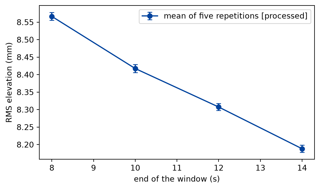
The standard error describes the repetitions. The window is a second choice: which seconds count as the steady wave train. The sweep moves the end of the window and keeps the start.

def window_sweep(measured):
    """The mean RMS elevation of the repetitions and its standard error for
    each end of the window, in mm."""
    window_scan = flume_analysis.window_sweep(measured)
    sigmas = [
        1e3
        * flume_analysis.estimate(
            flume_analysis.repetition_results(
                measured, (flume_analysis.WINDOW[0], end)
            )[0]
        ).sigma
        for end in window_scan.values
    ]
    return window_scan, sigmas

src/pbc/mechanics/experiments/automated_analysis_pipelines.py, lines 136 to 149, read from the repository when this page was built.

def draw_window_sweep(window_scan, sigmas) -> Figure:
    """The mean RMS elevation against the end of the window."""
    ends = window_scan.values
    window_fig, window_ax = plt.subplots(figsize=(6.4, 3.6))
    window_ax.errorbar(
        ends,
        1e3 * window_scan.results["rms"],
        yerr=sigmas,
        color=FIGURE_COLOURS[0],
        marker="o",
        capsize=3,
        label="mean of five repetitions [processed]",
    )
    window_ax.set_xlabel("end of the window (s)")
    window_ax.set_ylabel("RMS elevation (mm)")
    window_ax.legend()
    return window_fig

src/pbc/mechanics/experiments/automated_analysis_pipelines.py, lines 152 to 168, read from the repository when this page was built.

Plot of RMS elevation in millimetres against the end of the window in seconds, with four points joined by a line. The points fall from left to right, steeply at first. Each point has a vertical bar that is too small to see against the fall. — Figure 2: processed RMS elevation of the mean of five repetitions against the end of the analysis window. The bar is the standard error of the repetitions; the result moves with the window by far more than the bar.

The window was cut from the aligned records, and selecting a window is a step that makes the data processed, as the status says. The figure and the table show the sweep of the window against the spread of the repetitions:

def window_table(experiment: Experiment, window_scan, sigmas) -> float:
    """Record the table of the window ends; return the spread of the mean
    RMS elevation over them, in m."""
    spread = float(window_scan.results["rms"].max() - window_scan.results["rms"].min())
    experiment.table(
        "window-sweep",
        [
            (end, 1e3 * rms_value, s)
            for end, rms_value, s in zip(
                window_scan.values, window_scan.results["rms"], sigmas, strict=True
            )
        ],
        columns=[
            ("end of the window", "s", ".0f"),
            ("RMS elevation", "mm", ".2f"),
            ("standard error", "mm", ".2f"),
        ],
        caption="The window end, the mean RMS elevation of the repetitions, and its "
        "standard error, to two decimals.",
    )
    return spread

src/pbc/mechanics/experiments/automated_analysis_pipelines.py, lines 171 to 191, read from the repository when this page was built.

The window end, the mean RMS elevation of the repetitions, and its standard error, to two decimals.
end of the window (s)	RMS elevation (mm)	standard error (mm)
8	8.57	0.01
10	8.42	0.01
12	8.31	0.01
14	8.19	0.01

Experimentally supported (gauge five of the first wave condition, windows from five seconds to the ends shown): The change of the RMS elevation with the end of the window is 36 times the standard error of the five repetitions. The uncertainty of this result is the window, and a report that gave only the standard error would be too confident by that factor. Why the value falls as the window grows is a question about the experiment (a wave train that is still building up, reflections from the ends of the flume); the pipeline shows that it does, and does not say why.

The three numerical runs go through the same function, and the report puts each beside the measurement without merging them.

def model_comparison(experiment: Experiment, models, mean_rms):
    """The three numerical runs in the same window against the measurement;
    record the table and return their relative differences, in per cent."""
    runs = flume_analysis.model_results(models)
    rows = [
        (
            name,
            1e3 * run_rms,
            1e3 * (run_rms - mean_rms.mean),
            flume_analysis.agreement(mean_rms, run_rms),
            run_period,
        )
        for name, (run_rms, run_period) in runs.items()
    ]
    rel_diff = [100 * abs(run_rms / mean_rms.mean - 1) for run_rms, _ in runs.values()]
    experiment.table(
        "model-comparison",
        rows,
        columns=[
            ("run", "", "s"),
            ("RMS elevation", "mm", ".2f"),
            ("minus measurement", "mm", ".2f"),
            ("in standard errors", "", ".1f"),
            ("period", "s", ".2f"),
        ],
        caption="The three numerical runs in the same window, their RMS elevation "
        "relative to the measurement, and their period, to two decimals.",
    )
    return rel_diff

src/pbc/mechanics/experiments/automated_analysis_pipelines.py, lines 194 to 222, read from the repository when this page was built.

The three numerical runs in the same window, their RMS elevation relative to the measurement, and their period, to two decimals.
run	RMS elevation (mm)	minus measurement (mm)	in standard errors	period (s)
i-VoF (OpenFOAM)	8.06	-0.13	-12.5	1.50
M-sigma (MIKE 3)	7.98	-0.21	-20.2	1.50
D-SPH (DualSPHysics)	7.97	-0.22	-21.2	1.50

Experimentally supported (gauge five of the first wave condition, window as stated): All three runs have a smaller RMS elevation than the measurement, by 1.6 to 2.7 per cent, and their periods agree with it within the resolution of the window. The difference in standard errors is large, and it should not be read as a significance: the standard error leaves out the window and the alignment. The difference in millimetres is smaller than the change from the window, so the data show that the runs are slightly low, and do not say by how much.

The report of this problem is the same function of the same data, and it is compared with its own expectation:

def flume_expectation():
    """The report of the measured problem, checked against its committed
    expectation."""
    flume = flume_analysis.build_report()
    check_report(flume, EXPECTED_DIR / "flume-waves.txt")
    print(
        "lines that differ from the committed expectation:"
        f" {len(differences(flume, (EXPECTED_DIR / 'flume-waves.txt').read_text()))}"
    )

src/pbc/mechanics/experiments/automated_analysis_pipelines.py, lines 225 to 233, read from the repository when this page was built.

lines that differ from the committed expectation: 0

Limits

The first-order uncertainty and the Monte Carlo run treat the launch speed as the only uncertain input. The mass, the drag coefficient, the air density, and the angle have uncertainties of their own, and a real throw would carry them too; the pipeline takes one input to show the method.
The ball is a baseball with round values for its drag; the range is a statement about this simulation, not a measurement of a thrown ball.
The standard error of the repetitions assumes they are independent. They were aligned on another gauge, and an error of that alignment is common to all five. The standard error is therefore a lower bound, and the table of the window shows that it is not the dominant uncertainty anyway.
The window sweep varies one end of the window and nothing else. It does not show the effect of the start of the window, of the detrending, or of the spectral window, and it does not make the result “uncertain by the spread”: it says the result depends on a choice by at least that much.
The comparison with the runs is for one gauge and one wave condition of the committed sample. The sample is a subset of the dataset, and nothing here says how the runs behave at other gauges.
An expectation compares the shown text. A change that stays below the shown digits passes, and so does a pair of errors that cancel in the shown digits. It does not replace the tests of the code that computes the numbers.

Self-check. The report of the throw matches its committed expectation, and the build passes. Does it follow that the computed ranges are correct? Say what the match does show, and which check in this lesson speaks to correctness.

With scripts, you can record in this browser that you answered this question.

Solution to the self-check

No. The match shows that the pipeline gives the numbers it gave when the expectation was last accepted, to the digits shown, and that none of the reported quantities moved since. It would pass for a wrong range as long as the range had always been wrong in the same way. What speaks to correctness is a comparison with something independent of the code: the throw without drag has a closed form, and a test checks that the simulation agrees with it to a small fraction, and the Monte Carlo run checks the propagated uncertainty against a different calculation. The expectation protects those results against drift, which is a different job.

Exercises

Exercise 1. A better instrument. The launch speed is measured again with half the standard uncertainty. Compute the uncertainty of the range at the best angle of the fine sweep, and compare it with the one in the report. Is it half?

Solution to exercise 1

def halved_speed_uncertainty(best):
    """Exercise 1: the uncertainty of the range at the best angle with the
    speed uncertainty and with half of it."""

    def at_best(sigma):
        _, error = propagate(
            lambda v: analysis.throw_range(float(v), best), [SPEED], [sigma]
        )
        return float(error)

    full, halved = at_best(SPEED_SIGMA), at_best(SPEED_SIGMA / 2)
    print(
        f"uncertainty of the range: {full:.2f} m with the old speed uncertainty,"
        f" {halved:.2f} m with half of it, ratio {halved / full:.2f}"
    )

src/pbc/mechanics/experiments/automated_analysis_pipelines.py, lines 236 to 250, read from the repository when this page was built.

uncertainty of the range: 1.47 m with the old speed uncertainty, 0.74 m with half of it, ratio 0.50

The ratio is one half. To first order the uncertainty of the range is the derivative times the uncertainty of the speed, so it is proportional to it, and halving the input halves the result. A pipeline that propagates an uncertainty makes the answer to “what would a better instrument buy” a computation, not a guess.

Exercise 2. Change something and watch the expectation. The report was made with the fourth-order stepper and a step of a hundredth of a second. Compute the range at the best angle with explicit Euler at that step, and with the report’s setting. Does the committed report notice the difference?

Solution to exercise 2

def euler_against_the_reference(best):
    """Exercise 2: the range at the best angle with explicit Euler and with
    the fourth-order stepper of the pipeline."""
    euler = projectile_range(SPEED, best, analysis.MASS, analysis.DRAG, analysis.DT)
    reference = analysis.throw_range(SPEED, best)
    print(
        f"explicit Euler: {euler:.2f} m; fourth-order stepper: {reference:.2f} m;"
        f" difference {euler - reference:+.2f} m"
    )

src/pbc/mechanics/experiments/automated_analysis_pipelines.py, lines 253 to 261, read from the repository when this page was built.

explicit Euler: 62.79 m; fourth-order stepper: 62.68 m; difference +0.11 m

Explicit Euler has an error proportional to the step, and here it changes the range by a visible amount at the displayed precision. A report built with the Euler stepper would differ from the expectation on every range line, and the build would fail on them. That is the purpose: a change of a method is never silent, and the diff of the expectation shows its size.

Run this experiment

This page was built from commit 6417e2ff90258bd2d2ba21d217eb7666fd24f680 of the repository.

In a clone at that commit, with the project’s Python packages installed, this command runs the experiment of this page:

uv run --locked --no-dev python -m pbc.mechanics.experiments.automated_analysis_pipelines results

Files, tests, and every command

The files behind it:

site/lessons/mechanics/10-automated-analysis-pipelines/index.qmd: this page, with every code cell.
src/pbc/data/pipeline.py: code the experiment runs.
src/pbc/data/flume_analysis.py: code the experiment runs.
src/pbc/data/reports.py: code the experiment runs.
src/pbc/mechanics/analysis.py: code the experiment runs.
src/pbc/mechanics/experiments/automated_analysis_pipelines.py: code the experiment runs.
src/pbc/experiment.py: code the experiment runs.
reports/expected/projectile-range.txt: code the experiment runs.
reports/expected/flume-waves.txt: code the experiment runs.
tests/unit/test_pipeline.py: tests of that code.
tests/unit/test_automated_analysis_pipelines_experiment.py: tests of that code.

With Git and uv installed (see the setup page), run:

git clone https://github.com/taspinar/physics-by-construction.git
cd physics-by-construction
git checkout 6417e2ff90258bd2d2ba21d217eb7666fd24f680
uv sync --locked --no-dev
uv run --locked --no-dev python -m pbc.mechanics.experiments.automated_analysis_pipelines results

The experiment writes every figure of this page into results/, as <label>.png, and every number and table of the page, as the page shows it, into results/results.json. Its numbers match this page to the digits shown, and its figure files are the ones the page shows; digits beyond those can differ between machines, because floating-point libraries differ. Change the code of the experiment and run it again to see what changes.