Interference and resonance

Waves add: pulses pass through each other, a plucked string sounds at its mode frequencies, a push at one of them builds up without limit, a grid disperses what the equation does not, and two sources make a pattern.

Course

Waves and optics, lesson 2 of 3

Slot

W2, Interference and resonance

Methods

Simulation

Difficulty

Intermediate, level 2 of 3

What you’ll learn

• Use the linearity of the wave equation to build standing waves and modes from travelling ones
• Check the frequencies of a simulated string against the analytic mode frequencies
• Show a resonance, and measure the dispersion that a grid adds to a wave
• Predict the pattern of two coherent sources and check it by adding their waves

Prerequisites

The wave equation.

Before you begin

• Trigonometry: the sum of two sines, and the identity for the product of a sine and a cosine
• Complex numbers: the form exp(i x) of a wave and the modulus of a sum

Related

none

Previous

The wave equation

Next

Sound, resonance, and the Doppler effect

With scripts, this page keeps a record in your browser of whether you completed the lesson. Nothing is stored without them.

With scripts, this place suggests what to do next, with the reason, from the progress saved in your browser. Without them, follow the learning path.

Two ripples on a pond cross, and where they cross the water shows a pattern of calm and rough lines that neither ripple had. A guitar string, plucked in the middle or near the end, sounds the same note with a different colour. A wine glass sings when a singer holds the right pitch, and breaks when the pitch is held loudly. The lesson builds on one property of the wave equation of the previous lesson to explain all of them: its solutions add.

The lesson uses the program of that lesson as the instrument. It builds a standing wave from two travelling ones, finds the notes of a plucked string in the spectrum of a simulation and compares them with the analytic frequencies, drives the string at a mode and away from it, and measures what the grid does to the frequencies, which is a small error in this case and a real effect in a physical chain of beads. It ends with two sources whose waves are added one by one and compared with the formula of the pattern.

Assumptions

1. The medium is linear. The wave equation has the displacement and its derivatives to the first power only, so the sum of two solutions is a solution. That holds for small amplitudes. A string plucked hard, or sound at the volume of a jet engine, steepens its waves and makes new frequencies, and then the sum of two solutions is not a solution.
2. Fixed ends, a uniform string. Every mode frequency below follows from the two ends and the one speed $c$. A string with a heavier section, or a pipe with a bulge, has modes that are not whole multiples of one number.
3. No damping. A mode keeps its amplitude for ever, and a driven mode grows without a bound. Every real resonance is limited by loss, and the height and width of a resonance peak measure it.
4. Coherent sources of one wavelength, far from the screen. The pattern of two sources needs a fixed phase relation between them and one wavelength. Light from two bulbs has neither. The far-field formula needs the screen far from the sources compared with their separation.
5. The grid is fine enough. A wave of the wavelength of a few cells is not represented well, and the dispersion example measures how badly.
6. A sampled signal and a window. A frequency read from a simulation comes from a record of finite length, with the resolution that the length allows, refined by a fit; its error is of the order stated in the tables.

Adding waves

If $u_1$ and $u_2$ solve $u_{tt} = c^2 u_{xx}$, so does $a\,u_1 + b\,u_2$ for any numbers $a$ and $b$, because differentiation is linear. This is the principle of superposition. Its consequences are large. Two waves that meet do not change each other: each goes on as if the other were not there, and where they overlap the displacements add. The numerical scheme of the previous lesson is made of sums of values, so it is linear too, and its solution for a sum of starting shapes is the sum of the solutions, to round-off.

Standing waves and modes

A wave $\sin(kx - \omega t)$ travels to the right and $\sin(kx + \omega t)$ to the left, with $\omega = ck$. Their sum is, by the sum-to-product identity,

$$\sin(kx - \omega t) + \sin(kx + \omega t) = 2\,\sin(kx)\,\cos(\omega t).$$

This is a standing wave: a fixed shape $\sin kx$ whose size oscillates in time, with points that never move, the nodes, where $\sin kx = 0$. On a string of length $L$ with both ends fixed, an end is a node, so $kL$ is a whole multiple of $\pi$:

$$k_n = \frac{n\pi}{L}, \qquad f_n = \frac{\omega_n}{2\pi} = \frac{n\,c}{2L}, \qquad n = 1, 2, 3, \dots$$

These are the modes of the string, and $f_1$ is the fundamental. The frequencies are whole multiples of the first, which is why a string sounds as a note and not as noise. Any shape of the string at rest is a sum of modes, its sine series $\sum_n b_n \sin(n\pi x/L)$, and each term then oscillates at its own frequency. A string plucked at a distance $a$ from one end has

$$b_n = \frac{2L^2\,\sin(n\pi a/L)}{n^2\pi^2\,a\,(L - a)}$$

for a unit height. The amplitude falls as $1/n^2$, a plucked string has a mellow sound, and $b_n$ is zero for every mode that has a node where the string was plucked. Plucked at a third of its length, a string has no third mode.

Resonance

Push the string with a force that has the shape of mode $n$ and varies as $\cos\Omega t$. The amplitude $a$ of the mode follows an oscillator driven at the frequency $\Omega$, as the harmonic oscillator of the mechanics course did,

$$\ddot a + \omega_n^2\,a = \cos\Omega t \quad\Rightarrow\quad a(t) = \frac{\cos\Omega t - \cos\omega_n t}{\omega_n^2 - \Omega^2}$$

for a start at rest. The size is bounded and set by the distance between the two frequencies. When $\Omega \to \omega_n$ the numerator and denominator both go to zero, and the limit is

$$a(t) = \frac{t\,\sin\omega_n t}{2\,\omega_n},$$

which grows in proportion to the time without limit: a resonance. The force is always in step with the motion, so every cycle adds a push in the direction the string is moving, and no loss stops it in the model.

Dispersion from the grid

A mode of the grid with wavenumber $k$ oscillates, by the calculation of the previous lesson, at the angular frequency

$$\omega(k) = \frac{2}{\Delta t}\,\arcsin\!\left(C\,\sin\frac{k\,\Delta x}{2}\right),$$

which is close to $ck$ for waves long compared with the cell and falls below it for short ones. A wave whose frequency is not proportional to its wavenumber is dispersive: its phase speed $\omega/k$ depends on the wavelength. A packet of waves then travels at the group velocity $\mathrm{d}\omega/\mathrm{d}k$, not at the phase speed, and a pulse made of many wavelengths spreads out as its parts fall behind each other. The same formula describes a physical system. A chain of equal masses joined by equal springs, which is a model of a crystal, obeys the scheme with $\Delta t \to 0$, $\omega = (2c/\Delta x)\,\sin(k\Delta x/2)$ with $c$ set by the springs and the masses, and its waves disperse for the same reason: a wave shorter than a few spacings is not a wave of a continuous string.

Two sources

Two point sources with the same phase and the wavelength $\lambda$ lie a distance $d$ apart. At a far screen, the paths from them to a point at the angle $\theta$ from the normal differ by $d\sin\theta$. The waves arrive in phase, and add up, when the difference is a whole number of wavelengths, and cancel when it is a half-integer number of wavelengths. Adding the two amplitudes, $1 + e^{\mathrm{i}\,2\pi d\sin\theta/\lambda}$, and squaring the modulus gives the intensity

$$I(\theta) = 4\,I_1\,\cos^2\!\left(\frac{\pi d \sin\theta}{\lambda}\right),$$

with $I_1$ the intensity of one source. The bright fringes are at $\sin\theta = m\lambda/d$. The sum of intensities would be $2 I_1$ everywhere; the pattern averages to it, and moves the energy from the dark lines to the bright ones.

Code

The modes, the spectrum of a recording, and the sum of two sources are in pbc.waves.modes; the frequencies of the grid and the driven mode are in pbc.waves.wave.

def spectrum_peaks(
    signal: ArrayLike, dt: float, *, count: int, floor: float = 0.01
) -> Array:
    """The frequencies (Hz) of the ``count`` strongest peaks of the spectrum
    of ``signal`` sampled every ``dt`` seconds, lowest first.

    The signal is multiplied by a Hann window, zero-padded to eight times
    its length, and transformed; each peak is refined by the parabola
    through the logarithm of its magnitude and its two neighbours. A peak
    below ``floor`` times the strongest one is not a peak.
    """
    signal = np.asarray(signal, dtype=float)
    size = 8 * signal.size
    window = np.hanning(signal.size)
    magnitude = np.abs(np.fft.rfft((signal - signal.mean()) * window, size))
    df = 1.0 / (size * dt)
    inner = magnitude[1:-1]
    is_peak = (inner > magnitude[:-2]) & (inner >= magnitude[2:])
    index = np.nonzero(is_peak & (inner > floor * magnitude.max()))[0] + 1
    strongest = index[np.argsort(magnitude[index])[::-1][:count]]
    refined = []
    for i in np.sort(strongest):
        a, b, c = np.log(magnitude[i - 1 : i + 2])
        shift = 0.5 * (a - c) / (a - 2.0 * b + c)
        refined.append((i + shift) * df)
    return np.array(refined)

src/pbc/waves/modes.py, lines 51 to 76, read from the repository when this page was built.

def two_source_amplitude(
    angle: ArrayLike, *, separation: float, wavelength: float, distance: float
) -> Array:
    """The amplitude on a screen at the ``distance`` m from two coherent
    point sources ``separation`` m apart, in phase, summed wave by wave.

    The sources lie on the x axis at plus and minus half the separation.
    Each gives a wave exp(i k r) / r with k = 2 pi / wavelength, at its
    distance r from the point of the screen that lies at the ``angle`` (rad)
    from the y axis, seen from the middle between the sources. The two complex waves
    are added, and the modulus is returned. The sum is the superposition
    principle; no formula for the pattern is used.
    """
    angle = np.asarray(angle, dtype=float)
    k = 2.0 * np.pi / wavelength
    px = distance * np.sin(angle)
    py = distance * np.cos(angle)
    total = np.zeros(angle.shape, dtype=complex)
    for source in (-separation / 2.0, separation / 2.0):
        r = np.hypot(px - source, py)
        total += np.exp(1j * k * r) / r
    return np.abs(total)

src/pbc/waves/modes.py, lines 79 to 100, read from the repository when this page was built.

def numerical_angular_frequency(k: ArrayLike, *, c: float, dx: float, dt: float):
    """The angular frequency (rad/s) with which the scheme oscillates the
    mode of wavenumber ``k`` (rad/m) on a grid: from

        sin(omega dt / 2) = C sin(k dx / 2)

    the frequency is omega = (2 / dt) arcsin(C sin(k dx / 2)). It
    approaches c k as dx and dt go to zero, and equals it at C = 1.
    """
    courant = courant_number(c, dt, dx)
    argument = courant * np.sin(np.asarray(k) * dx / 2.0)
    if np.any(np.abs(argument) > 1.0):
        raise ValueError("the Courant number is too large: the mode does not oscillate")
    return 2.0 / dt * np.arcsin(argument)

src/pbc/waves/wave.py, lines 231 to 244, read from the repository when this page was built.

Worked examples

Pulses pass through each other

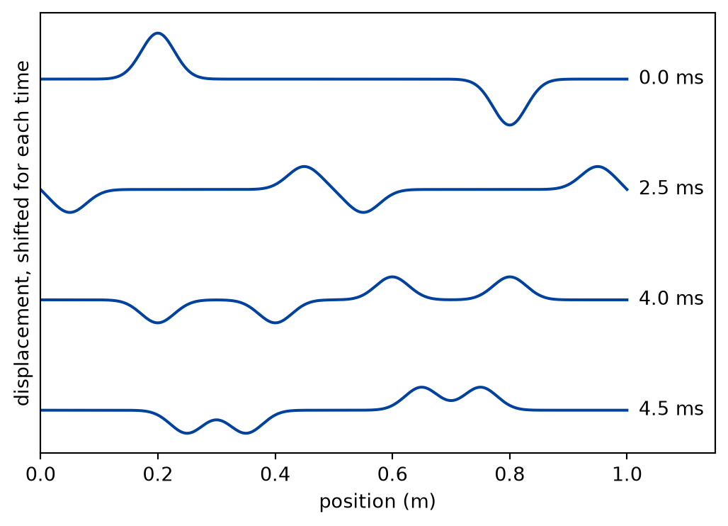
The string is 1 m long with the wave speed 100 m/s. Two pulses of the same shape are placed on it, one near each end and heading for the middle, one pointing up and one down. Both ends are fixed. The Courant number is one half, with four hundred cells.

LENGTH = 1.0  # string length, m
SPEED = 100.0  # wave speed, m/s

src/pbc/waves/experiments/interference_and_resonance.py, lines 40 to 41, read from the repository when this page was built.

LINEARITY_BOUND = 1e-12

src/pbc/waves/experiments/interference_and_resonance.py, line 44, read from the repository when this page was built.

def superposition():
    """Two pulses of opposite sign on 400 cells, run together and apart; the
    largest difference between the run of the sum and the sum of the runs."""
    cells = 400
    dx = LENGTH / cells
    dt = 0.5 * dx / SPEED
    x = grid(LENGTH, cells)

    def pulse(centre, sign):
        return sign * np.exp(-(((x - centre) / 0.04) ** 2))

    up = pulse(0.2, +1.0)
    down = pulse(0.8, -1.0)
    steps = round(0.0045 / dt)
    kwargs = dict(c=SPEED, dx=dx, dt=dt, n_steps=steps, every=1)
    both = solve(up + down, np.zeros_like(x), **kwargs)
    only_up = solve(up, np.zeros_like(x), **kwargs)
    only_down = solve(down, np.zeros_like(x), **kwargs)
    linearity_gap = error_norm(both.u, only_up.u + only_down.u)
    assert linearity_gap < LINEARITY_BOUND, (
        "the sum of two solutions is not the solution of the sum"
    )
    return x, both

src/pbc/waves/experiments/interference_and_resonance.py, lines 57 to 79, read from the repository when this page was built.

def draw_superposition(x, both) -> Figure:
    """The two pulses at four times, shifted for each time."""
    times = [0.0, 0.0025, 0.004, 0.0045]
    fig, ax = plt.subplots(figsize=(6.4, 4.2))
    for row, t in enumerate(times):
        j = int(np.argmin(np.abs(both.t - t)))
        ax.plot(x, both.u[j] - 2.4 * row, color="#00429d")
        ax.text(1.02, -2.4 * row, f"{both.t[j] * 1000:.1f} ms", va="center")
    ax.set_xlabel("position (m)")
    ax.set_ylabel("displacement, shifted for each time")
    ax.set_yticks([])
    ax.set_xlim(0, 1.15)
    return fig

src/pbc/waves/experiments/interference_and_resonance.py, lines 82 to 94, read from the repository when this page was built.

Figure 1: simulated Two pulses of opposite sign run towards each other. At the moment they overlap, the field is the sum and nearly cancels; afterwards each continues as if the other had not been there.

Numerically verified (two Gaussian pulses, fixed ends, Courant number one half): The field of two pulses released together equals the sum of the fields of each released alone. The largest difference between the two, over every node and every step of the run, is below 1e-12, which is round-off. The figure shows what that means: after they overlap, each pulse continues with its own shape and sign. The data are simulated, and the check is the linearity of the scheme, not a measurement of any real string.

The notes of a plucked string

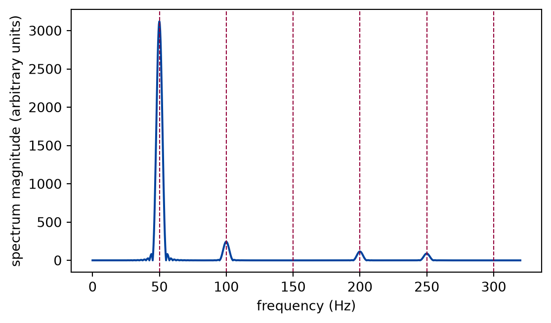
The string is plucked into a triangle at a third of its length, held at rest, and let go. The program records the displacement at one node, at forty-five hundredths of the length, for twenty periods of the fundamental, and the spectrum of the record is read.

MODE_TOLERANCE = 2e-3  # a chosen tolerance on the relative difference

src/pbc/waves/experiments/interference_and_resonance.py, line 47, read from the repository when this page was built.

def modes_run(experiment: Experiment):
    """A string plucked at a third, and the four strongest peaks of the
    spectrum at one point against the mode frequencies; record the table."""
    n_cells = 200
    dx = LENGTH / n_cells
    dt = 0.5 * dx / SPEED
    xs = grid(LENGTH, n_cells)
    steps = round(0.4 / dt)
    pluck = solve(
        triangle(xs, length=LENGTH, at=LENGTH / 3),
        np.zeros_like(xs),
        c=SPEED,
        dx=dx,
        dt=dt,
        n_steps=steps,
    )
    probe = round(0.45 * n_cells)
    record = pluck.u[:, probe]
    found = spectrum_peaks(record, dt, count=4)
    present = [1, 2, 4, 5]  # the third mode has a node at the pluck
    analytic = np.array([string_frequency(n, length=LENGTH, c=SPEED) for n in present])
    scheme = np.array(
        [
            numerical_angular_frequency(n * np.pi / LENGTH, c=SPEED, dx=dx, dt=dt)
            / (2 * np.pi)
            for n in present
        ]
    )
    deviation = np.abs(found - analytic) / analytic
    assert np.all(deviation < MODE_TOLERANCE), "a mode is not where the formula puts it"
    assert np.all(np.abs(found - scheme) / scheme < 1e-4), (
        "a peak is off the grid's own frequency"
    )
    assert abs(triangle_mode_amplitude(3, length=LENGTH, at=LENGTH / 3)) < 1e-12

    experiment.table(
        "modes-run",
        [
            (n, a, f, d * 100)
            for n, a, f, d in zip(present, analytic, found, deviation, strict=True)
        ],
        [
            ("mode", "", "d"),
            ("analytic n c / 2L", "Hz", ".2f"),
            ("simulated", "Hz", ".2f"),
            ("difference", "%", ".3f"),
        ],
        "The frequencies of the four strongest peaks of the spectrum of a plucked "
        "string, against the analytic mode frequencies, to two decimals.",
    )
    return record, dt, analytic, scheme, deviation

src/pbc/waves/experiments/interference_and_resonance.py, lines 97 to 147, read from the repository when this page was built.

The frequencies of the four strongest peaks of the spectrum of a plucked string, against the analytic mode frequencies, to two decimals.

mode	analytic n c / 2L (Hz)	simulated (Hz)	difference (%)
1	50.00	50.00	0.001
2	100.00	99.99	0.006
4	200.00	199.97	0.013
5	250.00	249.95	0.019

def draw_modes_spectrum(record, dt) -> Figure:
    """The spectrum of the plucked string with the mode frequencies."""
    size = 8 * record.size
    spectrum = np.abs(
        np.fft.rfft((record - record.mean()) * np.hanning(record.size), size)
    )
    frequency = np.arange(spectrum.size) / (size * dt)
    band = frequency < 320.0
    fig, ax = plt.subplots(figsize=(6.4, 3.6))
    ax.plot(frequency[band], spectrum[band], color="#00429d")
    for n in range(1, 7):
        ax.axvline(
            string_frequency(n, length=LENGTH, c=SPEED),
            color="#93003a",
            linestyle="--",
            linewidth=0.8,
        )
    ax.set_xlabel("frequency (Hz)")
    ax.set_ylabel("spectrum magnitude (arbitrary units)")
    return fig

src/pbc/waves/experiments/interference_and_resonance.py, lines 150 to 169, read from the repository when this page was built.

Figure 2: simulated The spectrum of the displacement of one node of a plucked string. The peaks stand at the whole multiples of the fundamental, marked by dashed lines; the third mode, which has a node at the pluck, is missing.

Numerically verified (a string plucked at a third, fixed ends, two hundred cells, twenty periods recorded): The peaks of the spectrum of a simulated plucked string lie at the analytic frequencies $n c / 2L$, and no peak lies at the third, which has a node at the pluck. The largest relative difference between a peak and the analytic frequency is 0.019 per cent, inside the chosen tolerance of 0.2 per cent. The grid accounts for it: the frequencies of the scheme itself differ from the analytic ones by up to 0.019 per cent for these four modes, and the peaks of the record agree with those. The data are simulated; the check is the formula.

A push at a mode and away from it

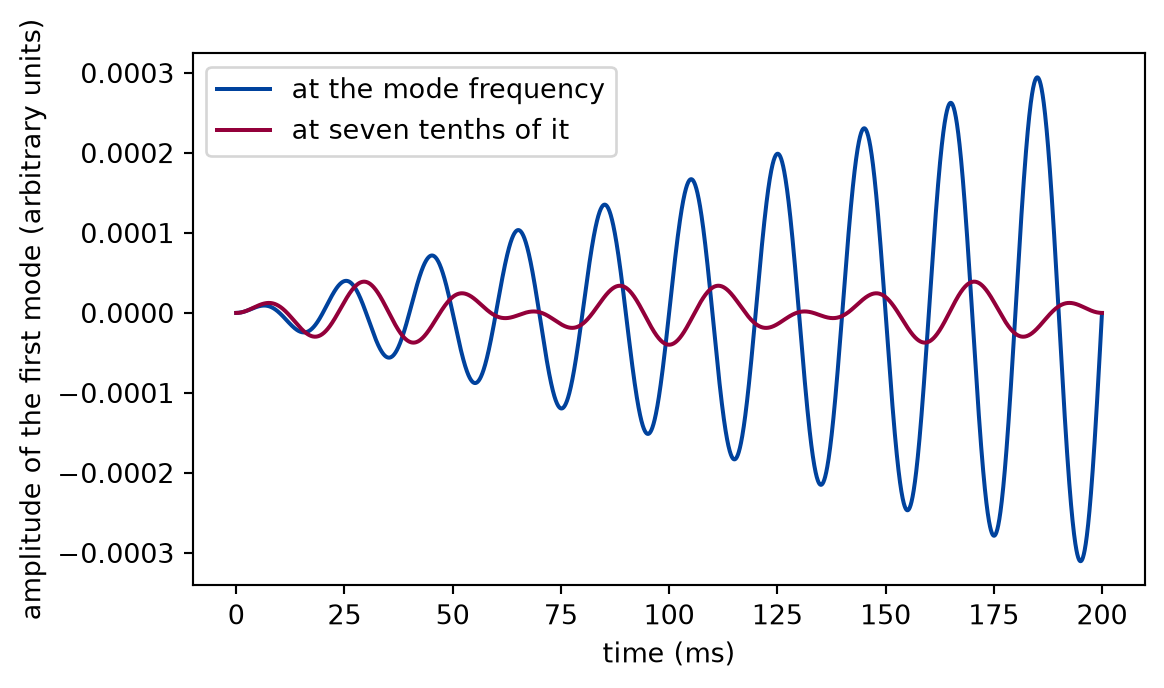
The same string is pushed with a force in the shape of the first mode, at the frequency of that mode and at seven tenths of it. The amplitude of the mode is read by projecting the field on the shape of the mode, and compared with the exact formula.

def resonance_run(experiment: Experiment):
    """The first mode driven at its frequency and at seven tenths of it,
    against the exact amplitude; record the table."""
    n_cells = 100
    dx = LENGTH / n_cells
    dt = 0.5 * dx / SPEED
    xs = grid(LENGTH, n_cells)
    shape = np.sin(np.pi * xs / LENGTH)
    omega1 = np.pi * SPEED / LENGTH
    steps = round(0.2 / dt)

    def driven(drive):
        result = solve(
            np.zeros_like(xs),
            np.zeros_like(xs),
            c=SPEED,
            dx=dx,
            dt=dt,
            n_steps=steps,
            forcing=lambda t: shape * np.cos(drive * t),
        )
        amplitude = result.u @ shape / (shape @ shape)
        exact = driven_mode_amplitude(
            result.t, length=LENGTH, n=1, c=SPEED, drive=drive
        )
        return result.t, amplitude, exact

    t_on, amp_on, exact_on = driven(omega1)
    t_off, amp_off, exact_off = driven(0.7 * omega1)
    gap_on = np.max(np.abs(amp_on - exact_on)) / np.max(np.abs(exact_on))
    gap_off = np.max(np.abs(amp_off - exact_off)) / np.max(np.abs(exact_off))
    assert gap_on < 0.02 and gap_off < 0.02
    growth = np.max(np.abs(amp_on[-steps // 5 :])) / np.max(
        np.abs(amp_on[: steps // 5])
    )

    experiment.table(
        "resonance-run",
        [
            ("at the mode frequency", np.max(np.abs(amp_on)), gap_on * 100),
            ("at seven tenths of it", np.max(np.abs(amp_off)), gap_off * 100),
        ],
        [
            ("drive", "", ""),
            ("largest amplitude of the mode in the run", "", ".2e"),
            ("largest gap from the exact amplitude", "% of its largest value", ".2f"),
        ],
        "The largest amplitude of the first mode in a run of ten periods, and how "
        "far the simulation is from the exact formula, for the two drives.",
    )
    return (t_on, amp_on, exact_on), (t_off, amp_off, exact_off), growth

src/pbc/waves/experiments/interference_and_resonance.py, lines 172 to 222, read from the repository when this page was built.

The largest amplitude of the first mode in a run of ten periods, and how far the simulation is from the exact formula, for the two drives.

drive	largest amplitude of the mode in the run	largest gap from the exact amplitude (% of its largest value)
at the mode frequency	3.10e-04	0.10
at seven tenths of it	3.97e-05	0.10

def draw_resonance(on, off) -> Figure:
    """The amplitude of the first mode under the two drives, simulated and
    exact."""
    t_on, amp_on, exact_on = on
    t_off, amp_off, exact_off = off
    fig, ax = plt.subplots(figsize=(6.4, 3.6))
    ax.plot(t_on * 1000, amp_on, color="#00429d", label="at the mode frequency")
    ax.plot(t_on * 1000, exact_on, color="#00429d", linestyle="--", linewidth=0.8)
    ax.plot(t_off * 1000, amp_off, color="#93003a", label="at seven tenths of it")
    ax.plot(t_off * 1000, exact_off, color="#93003a", linestyle="--", linewidth=0.8)
    ax.set_xlabel("time (ms)")
    ax.set_ylabel("amplitude of the first mode (arbitrary units)")
    ax.legend()
    return fig

src/pbc/waves/experiments/interference_and_resonance.py, lines 225 to 238, read from the repository when this page was built.

Figure 3: simulated The amplitude of the first mode of the driven string. At its own frequency the envelope grows in proportion to the time; away from it the amplitude beats at a fixed size. Dashed lines are the exact formulas.

Numerically verified (the first mode, fixed ends, one hundred cells, ten periods): A force at the frequency of a mode makes its amplitude grow in proportion to the time, and a force at another frequency leaves it bounded; the simulation follows both exact formulas. The amplitude in the last fifth of the run is 5.5 times the amplitude in the first fifth at resonance, while away from it the amplitude never exceeds 4.0e-05, in the same units, set by the distance of the two frequencies. In a real string the growth stops where loss balances the push, and this model has none.

What the grid does to a wave

The frequency of a standing mode is read from the zero crossings of the displacement at its first antinode, for modes from the longest on the string to the shortest the grid holds nearly, and compared with the analytic frequency and with the formula of the grid.

dispersion_cells = 100
mode_numbers = [1, 5, 10, 20, 40, 60, 80]

src/pbc/waves/experiments/interference_and_resonance.py, lines 242 to 243, read from the repository when this page was built.

def dispersion_run(experiment: Experiment):
    """The frequency of seven standing modes of the grid: analytic, from the
    dispersion relation of the scheme, and measured; record the table."""
    dx = LENGTH / dispersion_cells
    dt = 0.5 * dx / SPEED
    xs = grid(LENGTH, dispersion_cells)
    steps = round(0.3 / dt)
    rows = []
    for n in mode_numbers:
        result = solve(
            np.sin(n * np.pi * xs / LENGTH),
            np.zeros_like(xs),
            c=SPEED,
            dx=dx,
            dt=dt,
            n_steps=steps,
        )
        antinode = max(1, round(dispersion_cells / (2 * n)))
        measured = measured_frequency(result.u[:, antinode], result.t)
        k = n * np.pi / LENGTH
        formula = numerical_angular_frequency(k, c=SPEED, dx=dx, dt=dt) / (2 * np.pi)
        exact_f = SPEED * k / (2 * np.pi)
        rows.append((n, k * dx / np.pi, exact_f, formula, measured, measured / exact_f))
    agreement = max(abs(row[4] / row[3] - 1.0) for row in rows)
    assert agreement < 1e-3, "the measured frequency is not the one of the scheme"

    experiment.table(
        "dispersion-run",
        rows,
        [
            ("mode", "", "d"),
            ("wavenumber over the largest the grid holds", "", ".2f"),
            ("analytic", "Hz", ".1f"),
            ("formula of the grid", "Hz", ".1f"),
            ("measured", "Hz", ".1f"),
            ("measured over analytic", "", ".3f"),
        ],
        "The frequency of seven standing modes of the grid: analytic, from the "
        "dispersion relation of the scheme, and read from the zero crossings of a "
        "run, with the ratio of the measured to the analytic value.",
    )
    return rows, agreement

src/pbc/waves/experiments/interference_and_resonance.py, lines 247 to 288, read from the repository when this page was built.

The frequency of seven standing modes of the grid: analytic, from the dispersion relation of the scheme, and read from the zero crossings of a run, with the ratio of the measured to the analytic value.

mode	wavenumber over the largest the grid holds	analytic (Hz)	formula of the grid (Hz)	measured (Hz)	measured over analytic
1	0.01	50.0	50.0	50.0	1.000
5	0.05	250.0	249.8	249.8	0.999
10	0.10	500.0	498.5	498.5	0.997
20	0.20	1000.0	987.6	987.6	0.988
40	0.40	2000.0	1899.0	1899.0	0.950
60	0.60	3000.0	2651.1	2651.1	0.884
80	0.80	4000.0	3154.9	3154.9	0.789

Numerically verified (one hundred cells, Courant number one half, modes from the first to the eightieth): The frequencies of the scheme follow its dispersion relation, which departs from $\omega = ck$ for waves of a few cells. The measured frequency agrees with the formula of the grid to 2.6e-06 in relative terms, for every mode, and falls below the analytic frequency by 21 per cent for the highest mode shown, which has barely 2.5 cells per wavelength.

A packet shows the second consequence. A packet with a carrier of 1.2 radians per cell is released at rest on a longer string, and its right-going half travels for a few milliseconds; the speed of its centre is read from the displacement of the centre of its energy.

def packet_run():
    """A packet of short waves on the grid: the speed of its centre, the
    time it ran, and the group velocity of the grid."""
    n_cells = 400
    dx = LENGTH / n_cells
    dt = 0.5 * dx / SPEED
    xs = grid(LENGTH, n_cells)
    carrier = 1.2 / dx
    packet = wave_packet(xs, centre=0.25, width=0.05, k=carrier)
    steps = round(0.0025 / dt)
    packet_run = solve(
        packet, np.zeros_like(xs), c=SPEED, dx=dx, dt=dt, n_steps=steps, every=steps
    )
    right_half = packet_run.u[-1] * (xs > 0.3)
    packet_speed = (centroid(xs, right_half) - 0.25) / packet_run.t[-1]
    group = float(numerical_group_velocity(carrier, c=SPEED, dx=dx, dt=dt))
    assert abs(packet_speed / group - 1.0) < 0.02
    return packet_speed, packet_run.t[-1], group

src/pbc/waves/experiments/interference_and_resonance.py, lines 291 to 308, read from the repository when this page was built.

The centre of the packet moves at 86.0 m/s over 2.5 ms; the group velocity of the grid is 86.0 m/s, and the wave speed of the string is 100 m/s. Numerically verified (one packet, carrier of a few cells per wavelength, Courant number one half): A packet of short waves on the grid travels slower than the wave speed of the equation it solves, at the group velocity of the scheme. The error is not in the physics of the string, and it is a physical effect in a chain of beads: whether the dispersion is a defect of a method or a property of a medium depends on what the grid stands for.

Two sources

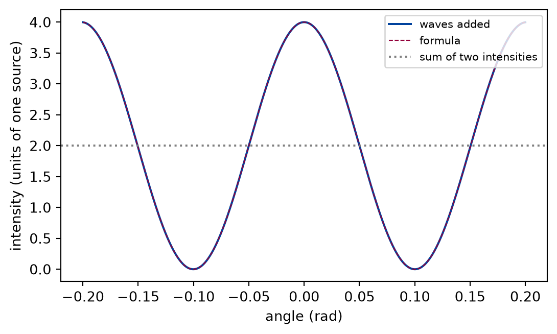
Two sources with the same phase, five wavelengths apart, are placed on a line. The waves $e^{\mathrm{i}kr}/r$ of the two are added at each of many points of a screen 20 km away, in units of the wavelength, and the intensity is compared with the formula of the far field.

wavelength = 1.0
separation = 5.0 * wavelength
distance = 20000.0 * wavelength
PATTERN_TOLERANCE = 5e-3  # in units of the intensity of one source

src/pbc/waves/experiments/interference_and_resonance.py, lines 50 to 53, read from the repository when this page was built.

def interference_run():
    """The intensity of two sources far away, added as waves and from the
    formula."""
    angle = np.linspace(-0.2, 0.2, 801)
    summed = two_source_amplitude(
        angle, separation=separation, wavelength=wavelength, distance=distance
    )
    intensity = (summed * distance) ** 2  # one source gives 1 at this distance
    formula = two_source_pattern(angle, separation=separation, wavelength=wavelength)
    pattern_gap = np.max(np.abs(intensity - formula))
    assert pattern_gap < PATTERN_TOLERANCE
    bright = np.arcsin(np.arange(-1, 2) * wavelength / separation)
    bright_values = two_source_pattern(
        bright, separation=separation, wavelength=wavelength
    )
    return angle, intensity, formula, pattern_gap, bright_values

src/pbc/waves/experiments/interference_and_resonance.py, lines 311 to 326, read from the repository when this page was built.

def draw_interference(angle, intensity, formula) -> Figure:
    """The intensity of two sources against the angle."""
    fig, ax = plt.subplots(figsize=(6.4, 3.6))
    ax.plot(angle, intensity, color="#00429d", label="waves added")
    ax.plot(
        angle, formula, color="#93003a", linestyle="--", linewidth=0.8, label="formula"
    )
    ax.axhline(2.0, color="gray", linestyle=":", label="sum of two intensities")
    ax.set_xlabel("angle (rad)")
    ax.set_ylabel("intensity (units of one source)")
    ax.legend(loc="upper right", fontsize=8)
    return fig

src/pbc/waves/experiments/interference_and_resonance.py, lines 329 to 340, read from the repository when this page was built.

Figure 4: simulated The intensity on a far screen of two coherent sources, in units of the intensity of one source: the waves added one by one (solid) and the cosine-squared formula (dashed). The dashed line at two is the sum of the two intensities.

Numerically verified (two sources five wavelengths apart, a screen twenty thousand wavelengths away): The intensity of two coherent sources, found by adding their waves, follows $4\cos^2(\pi d\sin\theta/\lambda)$ in the far field. The largest difference between the summed intensity and the formula is 1.1e-07 units of the intensity of one source, and the formula reaches 4 at the bright fringes, at angles that satisfy $\sin\theta = m\lambda/d$, twice the sum of the two intensities. Energy is not created: the pattern averages to that sum and moves energy from the dark lines to the bright ones. The data are simulated; the check is the formula.

Limits

• A linear, lossless model. Every real string, pipe, and glass has loss, which limits a resonance to a finite height and width; the lesson shows the limit without loss, in which growth has no end.
• Frequencies from a finite record. The spectrum has a finite resolution and the peak is refined by a fit. The agreement is of the order of a tenth of a per cent here and is not the accuracy of the scheme.
• Dispersion by the grid is not a measurement of a medium. The lesson measures the scheme’s dispersion and states its form. That a chain of beads has the same form is derived, not measured.
• Point sources, coherent and in phase. Sources of finite size, a broad range of wavelengths, or a changing phase wash the pattern out. Diffraction by a slit of finite width is a later lesson.

Self-check. Plucked at its middle, why does a string sound only the odd modes?

1. The even modes have a frequency that the string cannot reach.

   Every whole multiple of the fundamental is a mode of the string, odd or even; nothing prevents the string from oscillating at the even ones.

2. The even modes have a node at the middle, so a pluck there gives them no amplitude.

   Correct: $\sin(n\pi/2)$ is zero for even $n$, so $b_n = 0$ for them.

3. Plucking at the middle adds energy to the odd modes only.

   Plucking gives each mode the share that its shape has in the pluck. The even modes have a node at the middle, and the shape of the pluck, a point there, cannot excite them.

Solution to the self-check

The shape of a pluck at the middle is symmetric about the middle. Mode $n$ is symmetric for odd $n$ and antisymmetric for even $n$, so the symmetric pluck contains no even mode. This is the same statement as the zero of $\sin(n\pi a/L)$ at $a = L/2$.

Exercises

Exercise 1. A pipe closed at one end. A string with one end fixed and the other free has the modes $\sin((2n - 1)\pi x / 2L)$. Pluck the string at a fifth of its length, with the right end free, record a node at six tenths of its length for twice as long as before, and find the first three peaks. How do they compare with $(2n-1)\,c/4L$?

Hint 1 of 1 for exercise 1

The solver takes left and right. The first peak is the lowest.

Solution to exercise 1

def free_end():
    """Exercise 1: a string with one free end; the three strongest peaks of
    its spectrum and the formula."""
    n_cells = 200
    dx = LENGTH / n_cells
    dt = 0.5 * dx / SPEED
    xs = grid(LENGTH, n_cells)
    free = solve(
        triangle(xs, length=LENGTH, at=0.2 * LENGTH),
        np.zeros_like(xs),
        c=SPEED,
        dx=dx,
        dt=dt,
        n_steps=round(0.8 / dt),
        right="free",
    )
    peaks = spectrum_peaks(free.u[:, round(0.6 * n_cells)], dt, count=3, floor=0.05)
    expected = np.array([(2 * n - 1) * SPEED / (4 * LENGTH) for n in (1, 2, 3)])
    return peaks, expected

src/pbc/waves/experiments/interference_and_resonance.py, lines 343 to 361, read from the repository when this page was built.

The peaks are at 25.0, 75.0, 125.0 Hz and the formula gives 25.0, 75.0, 125.0 Hz. They are the odd multiples of the fundamental of a string half as long: the free end is an antinode, and a quarter of a wavelength fits in the length for the first mode.

Exercise 2. Beats. Two sources of nearly the same frequency, $f_1 = 100$ Hz and $f_2 = 104$ Hz, are heard together. How often does the loudness repeat?

Hint 1 of 1 for exercise 2

Add the two sines with the sum-to-product identity of the lesson.

Solution to exercise 2

def beats():
    """Exercise 2: two tones 4 Hz apart and their envelope."""
    f1, f2 = 100.0, 104.0
    t = np.linspace(0.0, 1.0, 20001)
    total = np.sin(2 * np.pi * f1 * t) + np.sin(2 * np.pi * f2 * t)
    envelope = 2 * np.abs(np.cos(np.pi * (f1 - f2) * t))
    beat_rate = abs(f1 - f2)
    return total, envelope, beat_rate

src/pbc/waves/experiments/interference_and_resonance.py, lines 364 to 371, read from the repository when this page was built.

The sum equals $2\cos(\pi(f_1 - f_2)t)\,\sin(\pi(f_1 + f_2)t)$: a tone at the mean frequency under an envelope that vanishes 4 times per second, the difference of the frequencies. The largest value of the sum over one second is 2.00, near the largest value 2 of the envelope.

Exercise 3. Where is the first dark line? For the two sources of the example, at what angle does the first dark line of the pattern lie?

Hint 1 of 1 for exercise 3

The path difference is half a wavelength.

Solution to exercise 3

def first_dark_fringe():
    """Exercise 3: the angle of the first dark fringe and the intensity
    there."""
    first_dark = np.arcsin(0.5 * wavelength / separation)
    value = two_source_pattern(first_dark, separation=separation, wavelength=wavelength)
    return first_dark, value

src/pbc/waves/experiments/interference_and_resonance.py, lines 374 to 379, read from the repository when this page was built.

The first dark line is at $\sin\theta = \lambda/2d$, which is 0.1002 rad here, and the formula gives the intensity 0.000 there, zero to round-off.

Run this experiment

This page was built from commit 6417e2ff90258bd2d2ba21d217eb7666fd24f680 of the repository.

In a clone at that commit, with the project’s Python packages installed, this command runs the experiment of this page:

uv run --locked --no-dev python -m pbc.waves.experiments.interference_and_resonance results

Files, tests, and every command

The files behind it:

• site/lessons/waves/02-interference-and-resonance/index.qmd: this page, with every code cell.
• src/pbc/waves/wave.py: code the experiment runs.
• src/pbc/waves/modes.py: code the experiment runs.
• src/pbc/waves/experiments/interference_and_resonance.py: code the experiment runs.
• src/pbc/experiment.py: code the experiment runs.
• tests/unit/test_waves.py: tests of that code.
• tests/unit/test_interference_and_resonance_experiment.py: tests of that code.

With Git and uv installed (see the setup page), run:

git clone https://github.com/taspinar/physics-by-construction.git
cd physics-by-construction
git checkout 6417e2ff90258bd2d2ba21d217eb7666fd24f680
uv sync --locked --no-dev
uv run --locked --no-dev python -m pbc.waves.experiments.interference_and_resonance results

The experiment writes every figure of this page into results/, as <label>.png, and every number and table of the page, as the page shows it, into results/results.json. Its numbers match this page to the digits shown, and its figure files are the ones the page shows; digits beyond those can differ between machines, because floating-point libraries differ. Change the code of the experiment and run it again to see what changes.