Sound, resonance, and the Doppler effect

Sound as a pressure wave computed on a grid: the resonances of open and closed pipes, a sweep through them, and the shift in pitch of a moving source or a moving listener, each checked against its formula.

Course

Waves and optics, lesson 3 of 3

Slot

W9, Sound waves, resonance, and the Doppler effect

Methods

Simulation

Difficulty

Intermediate, level 2 of 3

What you’ll learn

Compute the resonances of an open and of a closed pipe from the wave equation and check them against the analytic frequencies
Find the resonances of a pipe by sweeping the frequency of a driving force
Compute the pitch that a listener hears from a moving source and for a moving listener, and check it against both Doppler formulas

Prerequisites

The wave equation, Interference and resonance.

Before you begin

Calculus: partial derivatives, and the linearisation of a function about a point

Related

none

Previous

Interference and resonance

Next

Electric fields, superposition, and the potential

With scripts, this page keeps a record in your browser of whether you completed the lesson. Nothing is stored without them.

With scripts, this place suggests what to do next, with the reason, from the progress saved in your browser. Without them, follow the learning path.

A flute plays a lower note when all its holes are covered, and a longer organ pipe is lower than a short one. The siren of an ambulance drops in pitch at the moment it passes, though the siren sounds the same note throughout. Both are sound, and both can be computed with the wave equation of the first lesson of this course, if the field of the equation is read as the pressure of the air.

This lesson makes that reading, and then asks the two questions the opening raises. Which frequencies does a pipe of a given length answer to, and how does that depend on whether its ends are open or closed? And what does a listener hear when the source or the listener moves? The pipe is computed on a grid and the frequencies are read from the simulation. The motion is computed from the moment at which each crest of the wave leaves the source, which does not use the formula of the shift, and the heard frequency is counted from the signal. The formulas are in the lesson to be compared with. Nothing here records a sound or needs a microphone; the lesson is numerical, and its checks are the analytic limits.

Assumptions

A small perturbation of a gas at rest. The pressure and the density of the air differ from their rest values by a small fraction. Then the equations of the flow can be linearised, and they give the wave equation. A loud sound, near a jet, is not small, and travels faster than the linearised speed.
A uniform gas with one speed of sound. The speed $c$ is constant along the pipe and does not depend on the frequency; it depends on the temperature, and the lesson uses 343 m/s, the value of air at twenty degrees Celsius. A temperature that changes along the pipe would change the resonances.
Plane waves in a narrow pipe. The pressure depends on the position along the pipe only. That holds when the width of the pipe is small compared with the wavelength. It fails for the high notes of a wide pipe, and across a width the waves have modes of their own.
Ideal ends. An open end holds the pressure at its value outside. A closed end has no flow through it. A real open end radiates, and acts as if the pipe were a little longer; that is the end correction, and it is not in the model.
No loss. The simulated pipe rings for ever, and the response to a force at a resonance grows without limit. Real air loses energy to the walls and to radiation, which sets the width of every resonance.
Source and listener move on a line through the medium, slower than sound. The air is at rest, so that the speed of the source and the speed of the listener are measured against it. A source that is faster than the sound makes a shock, and the formulas of the shift stop.

The wave equation for sound

Take a gas of density $\rho_0$ at rest and ask for a small disturbance. Let the pressure be $p_0 + p$ and the velocity along the pipe $v$ . Two laws make the equations. The first is conservation of mass: gas that flows into a slab raises its density, $\partial \rho/\partial t = -\rho_0\,\partial v/\partial x$ . The second is Newton’s second law for the gas in the slab, in which the net force is the difference of the pressure on its two faces, $\rho_0\,\partial v/\partial t = -\partial p/\partial x$ . The gas compresses without exchanging heat with its surroundings on the time scale of the wave, so a change of the pressure is proportional to a change of the density, $p = c^2 \rho$ , which defines $c$ here: for an ideal gas $c^2 = \gamma p_0/\rho_0$ with $\gamma$ the ratio of the heat capacities. Differentiating the first law in time and the second in space and removing $v$ gives

$\frac{\partial^2 p}{\partial t^2} = c^2\,\frac{\partial^2 p}{\partial x^2},$

the wave equation of the first lesson, for the pressure. Everything of that lesson holds for sound: the solution of d’Alembert, the scheme, the Courant limit, the modes. What sound adds is the meaning of the ends.

At a closed end the gas cannot flow through the wall, $v = 0$ , and by the second law $\partial p/\partial x = 0$ : a free end of the field. At an open end the gas is free to move, and the pressure stays at the pressure outside, $p = 0$ : a fixed end of the field. A pipe is therefore a string with two ends of those kinds.

Resonances of a pipe

An open pipe of length $L$ is a string with two fixed ends, and its modes are those of the previous lesson,

$f_n = \frac{n\,c}{2L}, \qquad n = 1, 2, 3, \dots$

A pipe closed at one end has a free end and a fixed end. A mode has an antinode of the pressure at the closed end and a node at the open end, and a quarter of a wavelength fits in the length for the first one:

$f_n = \frac{(2n - 1)\,c}{4L}.$

The closed pipe sounds an octave lower than the open one of the same length, and has only the odd multiples of its lowest frequency, which is why a clarinet, which is closed at its reed end, has a different tone from a flute.

The Doppler shift

A source emits a tone of frequency $f_0$ . The crests of the wave leave the source one period $1/f_0$ apart and then travel at the speed $c$ , in the medium, whatever the source does.

If the source moves towards a listener at rest at the speed $v_s$ , each crest is emitted a distance $v_s/f_0$ closer than the one before, so the crests arrive spaced by $(c - v_s)/f_0$ , and the listener hears

$f = f_0\,\frac{c}{c - v_s}.$

If the listener moves towards a source at rest at the speed $v_o$ , the spacing of the crests is still $c/f_0$ , but the listener meets them faster, at the relative speed $c + v_o$ :

$f = f_0\,\frac{c + v_o}{c}.$

The two are not the same function: the medium is a reference, and it makes the motion of the source different from that of the listener. They agree to first order in $v/c$ , where both read $f_0\,(1 + v/c)$ , and differ in the second order. A speed that is negative is a motion away.

The computation from the moment of emission

The program does not use either formula. A crest that leaves the source at the time $\tau$ from its position $x_s(\tau)$ reaches the listener at the position $x_o(t)$ at the time $t$ if $t - \tau = |x_o(t) - x_s(\tau)|/c$ . For each $t$ the program finds the $\tau$ that satisfies it by bisection, and the signal at the listener is $\sin(2\pi f_0 \tau)$ . The heard frequency is then the number of periods of that signal divided by the time they take, counted from its zero crossings. Both formulas are a result of this calculation, and the lesson checks that they come out.

Code

The frequencies of a pipe are pipe_frequency, and the two formulas of the shift are source_shift and observer_shift. The calculation from the moment of emission is emission_time.

def pipe_frequency(n: int, *, length: float, c: float, closed_end: bool) -> float:
    """The frequency in Hz of resonance ``n`` (1, 2, ...) of a pipe of
    ``length`` m.

    Open at both ends: f_n = n c / (2 L), every harmonic. Closed at one end
    and open at the other: f_n = (2 n - 1) c / (4 L), the odd harmonics of
    the fundamental c / (4 L). The end correction of a real open end is not
    included (see the limits of lesson W9).
    """
    if n < 1 or length <= 0 or c <= 0:
        raise ValueError("need a resonance n >= 1, a positive length and speed")
    if closed_end:
        return (2 * n - 1) * c / (4.0 * length)
    return n * c / (2.0 * length)

src/pbc/waves/sound.py, lines 40 to 53, read from the repository when this page was built.

def emission_time(
    t: ArrayLike, source: Path, observer: Path, c: float, *, t_start: float = 0.0
) -> Array:
    """The time tau at which the signal that the observer receives at each
    time ``t`` left the source: the root of t - tau = |x_o(t) - x_s(tau)| / c.

    ``source`` and ``observer`` give the position (m) on the line at an
    array of times. Both must move slower than ``c``, and the signal must
    have left at or after ``t_start``. The root is found by bisection, which
    needs only that the left side minus the right side falls as tau
    increases, true for a source slower than the sound. A time before the
    first signal can arrive (including any ``t`` before ``t_start``) has no
    such root and raises ``ValueError``.
    """
    t = np.asarray(t, dtype=float)
    position = observer(t)
    first = source(np.full(t.shape, t_start))
    if np.any((t - t_start) - np.abs(position - first) / c < 0.0):
        raise ValueError(
            "no signal has arrived yet at some receive time: it is before t_start"
            " plus the travel time from the source"
        )
    low = np.full(t.shape, t_start)
    high = t.copy()
    for _ in range(80):
        middle = 0.5 * (low + high)
        # t - middle is the travel time available; the signal needs the
        # distance divided by c. Early tau leaves too little time to spare.
        spare = (t - middle) - np.abs(position - source(middle)) / c
        low = np.where(spare > 0.0, middle, low)
        high = np.where(spare > 0.0, high, middle)
    return 0.5 * (low + high)

src/pbc/waves/sound.py, lines 73 to 104, read from the repository when this page was built.

def measured_frequency(signal: ArrayLike, t: ArrayLike) -> float:
    """The frequency (Hz) of a tone, from its rising zero crossings: the
    number of periods between the first and the last crossing, divided by
    the time between them. A crossing is placed by linear interpolation
    between the two samples around it."""
    signal = np.asarray(signal, dtype=float)
    t = np.asarray(t, dtype=float)
    up = np.nonzero((signal[:-1] < 0.0) & (signal[1:] >= 0.0))[0]
    if up.size < 2:
        raise ValueError("fewer than two rising zero crossings in the signal")
    fraction = -signal[up] / (signal[up + 1] - signal[up])
    crossings = t[up] + fraction * (t[up + 1] - t[up])
    return float((up.size - 1) / (crossings[-1] - crossings[0]))

src/pbc/waves/modes.py, lines 113 to 125, read from the repository when this page was built.

Worked examples

The notes of an open and of a closed pipe

The pipe is 0.8 m long. The pressure inside it starts as a triangular profile that peaks at a fifth of the length, the pipe is left alone for 0.4 s, and the pressure is recorded at one point. A shape that is not a single mode contains many, so the pipe answers with its own frequencies. The first three peaks of the spectrum are read, once for a pipe that is open at both ends and once for one closed at its right end. The grid has one hundred sixty cells and the Courant number is one half.

LENGTH = 0.8  # pipe length, m
SOUND = SPEED_OF_SOUND  # speed of sound, m/s
PIPE_TOLERANCE = 1e-3  # a chosen tolerance on the relative difference

src/pbc/waves/experiments/sound_and_the_doppler_effect.py, lines 31 to 33, read from the repository when this page was built.

def pipe_run(experiment: Experiment):
    """A pulse in a pipe open at both ends and in one closed at one end, and
    the first three peaks of the spectrum against the analytic resonances;
    record the table and return its rows and the largest difference."""
    cells = 160
    dx = LENGTH / cells
    dt = 0.5 * dx / SOUND
    xs = grid(LENGTH, cells)
    pulse = triangle(xs, length=LENGTH, at=0.2 * LENGTH)
    steps = round(0.4 / dt)
    stride = 4  # the field is recorded every fourth step

    pipes = {
        "open at both ends": dict(
            left="fixed", right="fixed", closed=False, probe=0.45
        ),
        "closed at the right end": dict(
            left="fixed", right="free", closed=True, probe=0.6
        ),
    }
    pipe_rows = []
    worst_pipe = 0.0
    for name, setup in pipes.items():
        result = solve(
            pulse,
            np.zeros_like(xs),
            c=SOUND,
            dx=dx,
            dt=dt,
            n_steps=steps,
            every=stride,
            left=setup["left"],
            right=setup["right"],
        )
        signal = result.u[:, round(setup["probe"] * cells)]
        found = spectrum_peaks(signal, stride * dt, count=3, floor=0.05)
        for n, f in zip((1, 2, 3), found, strict=True):
            expected = pipe_frequency(
                n, length=LENGTH, c=SOUND, closed_end=setup["closed"]
            )
            worst_pipe = max(worst_pipe, abs(f / expected - 1.0))
            pipe_rows.append((name, n, expected, f, (f / expected - 1.0) * 100))
    assert worst_pipe < PIPE_TOLERANCE, "a resonance is not where the formula puts it"

    experiment.table(
        "pipe-run",
        pipe_rows,
        [
            ("pipe", "", ""),
            ("resonance", "", "d"),
            ("analytic", "Hz", ".1f"),
            ("simulated", "Hz", ".1f"),
            ("difference", "%", ".4f"),
        ],
        "The first three resonances of a pipe of the stated length, open at both "
        "ends and closed at one, against the analytic frequencies, and the "
        "percentage difference.",
    )
    return pipe_rows, worst_pipe

src/pbc/waves/experiments/sound_and_the_doppler_effect.py, lines 43 to 101, read from the repository when this page was built.

The first three resonances of a pipe of the stated length, open at both ends and closed at one, against the analytic frequencies, and the percentage difference.
pipe	resonance	analytic (Hz)	simulated (Hz)	difference (%)
open at both ends	1	214.4	214.4	-0.0012
open at both ends	2	428.8	428.7	-0.0048
open at both ends	3	643.1	643.1	-0.0108
closed at the right end	1	107.2	107.2	-0.0003
closed at the right end	2	321.6	321.6	-0.0027
closed at the right end	3	535.9	535.9	-0.0075

Numerically verified (a uniform pipe, ideal ends, one hundred sixty cells, a record of four tenths of a second): The first three resonances of a simulated pipe agree with $n c/2L$ for the pipe open at both ends and with $(2n-1)c/4L$ for the pipe closed at one end. The largest difference is 0.0108 per cent, inside the chosen tolerance of 0.1 per cent. The lowest resonance of the closed pipe is 107.2 Hz, half that of the open one at 214.4 Hz, and its next resonance is 3.00 times the lowest, the odd multiple that a closed pipe has in place of the even one. The data are simulated, and the check is the analytic frequency.

Sweeping the frequency of a push

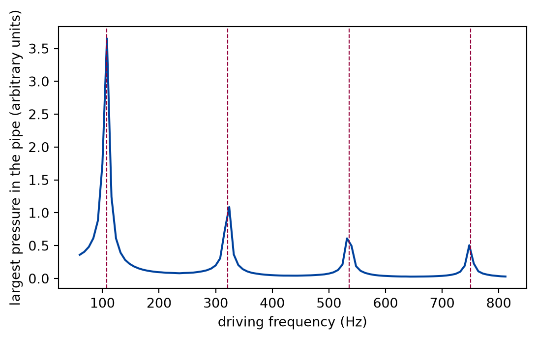
A pipe in use is not struck by a pulse but driven. Here the closed pipe is pushed at its closed end by a force $\cos\Omega t$ for a tenth of a second, and the largest pressure anywhere in the pipe during that time is recorded, for many values of $\Omega$ . The grid has forty cells.

def sweep_run(experiment: Experiment):
    """The closed pipe driven next to its closed end over a sweep of
    frequencies: its largest response, and the four peaks against the
    resonances; record the table."""
    cells = 40
    dx = LENGTH / cells
    dt = 0.5 * dx / SOUND
    xs = grid(LENGTH, cells)
    steps = round(0.1 / dt)
    push = np.zeros_like(xs)
    push[-2] = 1e6  # a push on the node next to the closed end, in m / s^2
    frequencies = np.arange(60.0, 820.0, 8.0)
    response = []
    for f in frequencies:
        omega = 2 * np.pi * f
        driven = solve(
            np.zeros_like(xs),
            np.zeros_like(xs),
            c=SOUND,
            dx=dx,
            dt=dt,
            n_steps=steps,
            every=5,
            left="fixed",
            right="free",
            forcing=lambda t: push * np.cos(omega * t),  # noqa: B023, used at once
        )
        response.append(np.max(np.abs(driven.u)))
    response = np.array(response)
    local = [
        i
        for i in range(1, len(response) - 1)
        if response[i] > response[i - 1]
        and response[i] >= response[i + 1]
        and response[i] > 0.05 * response.max()  # a peak, not a ripple
    ]
    peak_frequencies = frequencies[local][:4]
    closed = np.array(
        [
            pipe_frequency(n, length=LENGTH, c=SOUND, closed_end=True)
            for n in (1, 2, 3, 4)
        ]
    )
    spacing = float(frequencies[1] - frequencies[0])
    assert len(peak_frequencies) == 4
    assert np.all(np.abs(peak_frequencies - closed) <= spacing), (
        "a peak is off a resonance"
    )

    experiment.table(
        "sweep-run",
        [
            (n, a, p, p - a)
            for n, a, p in zip((1, 2, 3, 4), closed, peak_frequencies, strict=True)
        ],
        [
            ("resonance", "", "d"),
            ("analytic", "Hz", ".1f"),
            ("peak of the sweep", "Hz", ".0f"),
            ("difference", "Hz", ".1f"),
        ],
        "The four peaks of the response of the closed pipe to a sweep of the "
        "driving frequency in steps of the stated spacing, against the analytic "
        "resonances.",
    )
    return frequencies, response, closed, spacing

src/pbc/waves/experiments/sound_and_the_doppler_effect.py, lines 104 to 169, read from the repository when this page was built.

The four peaks of the response of the closed pipe to a sweep of the driving frequency in steps of the stated spacing, against the analytic resonances.
resonance	analytic (Hz)	peak of the sweep (Hz)	difference (Hz)
1	107.2	108	0.8
2	321.6	324	2.4
3	535.9	532	-3.9
4	750.3	748	-2.3

def draw_sweep(frequencies, response, closed) -> Figure:
    """The response of the closed pipe against the driving frequency."""
    fig, ax = plt.subplots(figsize=(6.4, 3.6))
    ax.plot(frequencies, response, color="#00429d")
    for f in closed:
        ax.axvline(f, color="#93003a", linestyle="--", linewidth=0.8)
    ax.set_xlabel("driving frequency (Hz)")
    ax.set_ylabel("largest pressure in the pipe (arbitrary units)")
    return fig

src/pbc/waves/experiments/sound_and_the_doppler_effect.py, lines 172 to 180, read from the repository when this page was built.

Line plot of the response against driving frequency from sixty to nine hundred hertz. Four sharp peaks rise from a low background, near one hundred, three hundred twenty, five hundred forty and seven hundred fifty hertz. Dashed vertical lines mark the analytic resonances through the tops of the peaks. — Figure 1: simulated The largest pressure in a closed pipe during a tenth of a second of driving, against the driving frequency. Peaks stand at the analytic resonances, marked by dashed lines, and the response between them is small.

Numerically verified (a closed pipe, forty cells, a tenth of a second of driving, steps of the stated spacing): A pipe driven at a range of frequencies answers at its resonances, the frequencies of its modes. Each of the four peaks of the sweep lies within one step of the sweep, 8 Hz, of the analytic resonance, which is all that a sweep with steps of that size can say. The width of a peak is set by the length of the drive, 10 Hz, since a driver that acts for a time $T$ cannot tell two frequencies apart by less than about $1/T$ ; in a real pipe the loss sets the width instead.

The pitch of a moving source and of a moving listener

The tone is 440 Hz. The listener is at rest at the origin while the source starts 300 m away on the line and moves towards the listener with each of the speeds in the table, and with the negative of each for a source that moves away. Then the roles are exchanged: the source is at rest, and the listener moves. The signal is computed for the interval from one and a half to two seconds after the start, which holds hundreds of periods, and the frequency is counted from the zero crossings.

F0 = 440.0  # frequency of the tone, Hz
START = 300.0  # starting distance, m
times = np.linspace(1.5, 2.0, 100_000)
DOPPLER_TOLERANCE = 1e-4  # a chosen tolerance on the relative difference

src/pbc/waves/experiments/sound_and_the_doppler_effect.py, lines 36 to 39, read from the repository when this page was built.

def at_rest(t):
    return np.zeros_like(t)

src/pbc/waves/experiments/sound_and_the_doppler_effect.py, lines 183 to 184, read from the repository when this page was built.

def source_moving(speed):
    return lambda t: -START + speed * t

src/pbc/waves/experiments/sound_and_the_doppler_effect.py, lines 187 to 188, read from the repository when this page was built.

def observer_moving(speed):
    return lambda t: START - speed * t

src/pbc/waves/experiments/sound_and_the_doppler_effect.py, lines 191 to 192, read from the repository when this page was built.

def heard(source, observer):
    return measured_frequency(
        received_signal(times, F0, source, observer, SOUND), times
    )

src/pbc/waves/experiments/sound_and_the_doppler_effect.py, lines 195 to 198, read from the repository when this page was built.

def doppler_run(experiment: Experiment):
    """The frequency heard from a moving source and by a moving listener at
    six speeds, computed and from the formula; record the table."""
    speeds = np.array([-120.0, -60.0, -30.0, 30.0, 60.0, 120.0])
    from_source = np.array([heard(source_moving(v), at_rest) for v in speeds])
    from_observer = np.array([heard(at_rest, observer_moving(v)) for v in speeds])
    formula_source = np.array([source_shift(F0, SOUND, v) for v in speeds])
    formula_observer = np.array([observer_shift(F0, SOUND, v) for v in speeds])
    gap_source = np.max(np.abs(from_source / formula_source - 1.0))
    gap_observer = np.max(np.abs(from_observer / formula_observer - 1.0))
    assert max(gap_source, gap_observer) < DOPPLER_TOLERANCE

    experiment.table(
        "doppler-run",
        list(
            zip(
                speeds,
                from_source,
                formula_source,
                from_observer,
                formula_observer,
                strict=True,
            )
        ),
        [
            ("speed towards", "m/s", ".0f"),
            ("moving source, computed", "Hz", ".2f"),
            ("moving source, formula", "Hz", ".2f"),
            ("moving listener, computed", "Hz", ".2f"),
            ("moving listener, formula", "Hz", ".2f"),
        ],
        "The frequency heard from a tone of the stated frequency, for a source and "
        "for a listener that move at the stated speed, towards (positive) or away "
        "(negative), computed from the moment of emission and from the formula.",
    )
    return speeds, from_source, from_observer, max(gap_source, gap_observer)

src/pbc/waves/experiments/sound_and_the_doppler_effect.py, lines 201 to 236, read from the repository when this page was built.

The frequency heard from a tone of the stated frequency, for a source and for a listener that move at the stated speed, towards (positive) or away (negative), computed from the moment of emission and from the formula.
speed towards (m/s)	moving source, computed (Hz)	moving source, formula (Hz)	moving listener, computed (Hz)	moving listener, formula (Hz)
-120	325.96	325.96	286.06	286.06
-60	374.49	374.49	363.03	363.03
-30	404.61	404.61	401.52	401.52
30	482.17	482.17	478.48	478.48
60	533.29	533.29	516.97	516.97
120	676.77	676.77	593.94	593.94

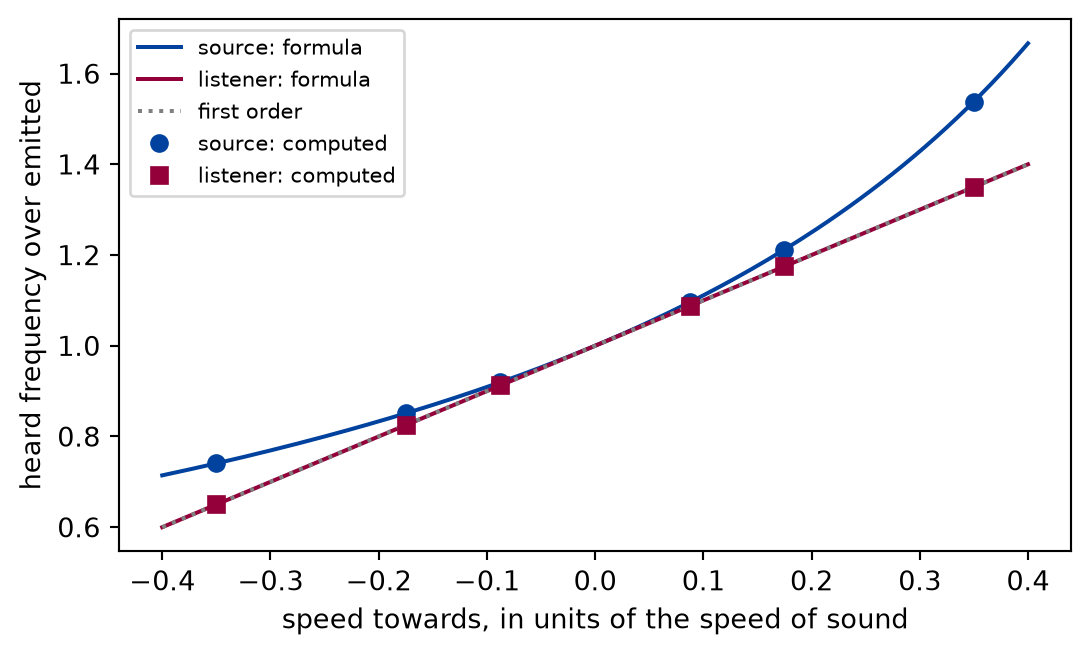
def draw_doppler(speeds, from_source, from_observer) -> Figure:
    """The heard frequency over the emitted against the speed, formulas and
    computed points."""
    v = np.linspace(-0.4, 0.4, 161) * SOUND
    fig, ax = plt.subplots(figsize=(6.4, 3.6))
    ax.plot(
        v / SOUND,
        [source_shift(F0, SOUND, s) / F0 for s in v],
        color="#00429d",
        label="source: formula",
    )
    ax.plot(
        v / SOUND,
        [observer_shift(F0, SOUND, s) / F0 for s in v],
        color="#93003a",
        label="listener: formula",
    )
    ax.plot(v / SOUND, 1 + v / SOUND, color="gray", linestyle=":", label="first order")
    ax.plot(
        speeds / SOUND, from_source / F0, "o", color="#00429d", label="source: computed"
    )
    ax.plot(
        speeds / SOUND,
        from_observer / F0,
        "s",
        color="#93003a",
        label="listener: computed",
    )
    ax.set_xlabel("speed towards, in units of the speed of sound")
    ax.set_ylabel("heard frequency over emitted")
    ax.legend(fontsize=8)
    return fig

src/pbc/waves/experiments/sound_and_the_doppler_effect.py, lines 239 to 270, read from the repository when this page was built.

Plot of the frequency ratio against the speed as a fraction of the speed of sound, from minus point four to plus point four. Two rising curves, one for the source that bends upward faster at positive speed, one for the listener that is a straight line. Markers lie on both curves. A dotted line shows the first-order straight line, one plus the speed fraction, tangent to both at zero. — Figure 2: simulated The ratio of the heard frequency to the emitted one against the speed of the source (blue) or of the listener (red) as a fraction of the speed of sound. The curves are the formulas and the markers are computed from the moment of emission. They coincide at small speeds and part at large ones.

Numerically verified (a tone, motion on a line through still air at speeds up to a third of the speed of sound): The frequency heard from a moving source follows $f_0 c/(c - v_s)$ , and the frequency heard by a moving listener follows $f_0 (c + v_o)/c$ , to a relative difference below the tolerance. The largest relative difference between the computed and the formula value is 6.0e-11, inside the chosen tolerance of 1e-04. At the largest speed shown the two cases differ: the source gives 676.8 Hz and the listener 593.9 Hz, though the relative speed of the two is the same. The medium decides which of the two moves. At small speeds the two curves and the straight line of the first order are the same within the thickness of the line, as the figure shows. The data are simulated, and the check is the two formulas.

Limits

Plane waves and ideal ends only. A real pipe has a radiating open end, which makes it act longer by a length of the order of its radius, walls that lose energy, and a mouthpiece or a reed that is not an ideal end. The resonances of a real instrument are close to these and not equal.
The Doppler shift is computed from the moment of emission, not from the grid. That makes it independent of the formulas and of the numerical scheme, and it also means that the lesson does not show a moving source on the grid, where it would need an interpolated source and a finer grid.
Motion along the line between source and listener. For another direction, the speed that matters is the component along the line from the source to the listener, which changes as they pass each other. The jump in pitch of a passing siren is then a curve, not a step.
Subsonic motion in still air. A moving medium, a wind, changes the speed of the signal; a source faster than sound has no heard frequency in the formula and makes a shock wave.
Numbers of the sweep are of the sweep. The peaks are located to the step of the sweep, and their width is that of the drive; the sweep does not measure a quality factor.

Self-check. A source and a listener approach each other, each moving at the same speed through the air. Is the pitch heard the same as when only the source moves at that speed?

Yes. Only the relative speed of the two matters.

Not for sound: the medium is a reference. The two situations have the same relative speed and give different pitches, which is the difference between the two formulas of the lesson.
No. The two effects add, and the pitch is higher than for the source alone.

Correct: the source shortens the spacing of the crests and the listener meets them faster. The pitch is $f_0 (c + v_o)/(c - v_s)$ , larger than either factor alone.
No. The pitch is lower, because the listener moves against the sound.

A listener that moves towards the source meets the crests more often, which raises the pitch, not lowers it.

Solution to the self-check

The source changes the spacing of the crests in the air, to $(c - v_s)/f_0$ , and the listener changes how fast it meets them, $c + v_o$ instead of $c$ . The two factors multiply: $f = f_0\,(c + v_o)/(c - v_s)$ . For equal speeds $v$ this is $f_0 (c + v)/(c - v)$ , above both $f_0 c/(c - v)$ and $f_0 (c + v)/c$ .

Exercises

Exercise 1. An ambulance. A siren of 700 Hz on an ambulance that drives at 25 m/s towards a pedestrian at rest. What does the pedestrian hear as it approaches, and what after it has passed and moves away?

Hint 1 of 1 for exercise 1

Use the formula for a moving source, with a negative speed for a motion away.

Solution to exercise 1

def siren():
    """Exercise 1: a siren of 700 Hz passing at 25 m/s."""
    tone = 700.0
    approaching = source_shift(tone, SOUND, 25.0)
    receding = source_shift(tone, SOUND, -25.0)
    drop = approaching - receding
    return approaching, receding, drop

src/pbc/waves/experiments/sound_and_the_doppler_effect.py, lines 273 to 279, read from the repository when this page was built.

The pedestrian hears 755.0 Hz as the ambulance approaches and 652.4 Hz after it has passed, a drop of 102.6 Hz. The ratio of the two pitches is 1.157, about 2.5 semitones.

Exercise 2. A pipe for a note. How long must a pipe closed at one end be for its lowest resonance to be the note of 440 Hz, and how long if it is open at both ends?

Hint 1 of 1 for exercise 2

Solve the formula of the lowest resonance for the length.

Solution to exercise 2

def pipes_for_a():
    """Exercise 2: the lengths of a closed and of an open pipe whose lowest
    resonance is 440 Hz."""
    closed_length = SOUND / (4 * 440.0)
    open_length = SOUND / (2 * 440.0)
    check = pipe_frequency(1, length=closed_length, c=SOUND, closed_end=True)
    return closed_length, open_length, check

src/pbc/waves/experiments/sound_and_the_doppler_effect.py, lines 282 to 288, read from the repository when this page was built.

The closed pipe is 19.5 cm long and the open one 39.0 cm: twice as long, because a closed pipe holds a quarter of a wavelength and an open one half. The formula for the closed pipe returns 440.0 Hz for the length found. A real pipe is a little shorter, by the end correction that the model leaves out.

Exercise 3. A resonance that the profile does not excite. In the first example, put the peak of the profile at the middle of the open pipe. Which of its resonances are missing from the spectrum, and why?

Hint 1 of 1 for exercise 3

Look at the shape of the modes of the pipe at its middle.

Solution to exercise 3

def plucked_in_the_middle():
    """Exercise 3: a pulse in the middle of the open pipe; its two strongest
    peaks and the distance of the nearest from the second resonance."""
    cells = 160
    dx = LENGTH / cells
    dt = 0.5 * dx / SOUND
    xs = grid(LENGTH, cells)
    centred = solve(
        triangle(xs, length=LENGTH, at=LENGTH / 2),
        np.zeros_like(xs),
        c=SOUND,
        dx=dx,
        dt=dt,
        n_steps=round(0.4 / dt),
        every=4,
    )
    found = spectrum_peaks(
        centred.u[:, round(0.17 * cells)], 4 * dt, count=2, floor=0.05
    )
    second = pipe_frequency(2, length=LENGTH, c=SOUND, closed_end=False)
    nearest = float(np.min(np.abs(found - second)))
    return found, second, nearest

src/pbc/waves/experiments/sound_and_the_doppler_effect.py, lines 291 to 312, read from the repository when this page was built.

The two strongest peaks are at 214.4, 643.1 Hz, the first and the third multiples of the lowest resonance 214.4 Hz, and none lies near the second resonance at 428.8 Hz: the nearest peak is 214 Hz away. The even modes have a node at the middle of the pipe, so a profile that is symmetric about it cannot excite them.

Run this experiment

This page was built from commit 6417e2ff90258bd2d2ba21d217eb7666fd24f680 of the repository.

In a clone at that commit, with the project’s Python packages installed, this command runs the experiment of this page:

uv run --locked --no-dev python -m pbc.waves.experiments.sound_and_the_doppler_effect results

Files, tests, and every command

The files behind it:

site/lessons/waves/03-sound-and-the-doppler-effect/index.qmd: this page, with every code cell.
src/pbc/waves/wave.py: code the experiment runs.
src/pbc/waves/modes.py: code the experiment runs.
src/pbc/waves/sound.py: code the experiment runs.
src/pbc/waves/experiments/sound_and_the_doppler_effect.py: code the experiment runs.
src/pbc/experiment.py: code the experiment runs.
tests/unit/test_waves.py: tests of that code.
tests/unit/test_sound_and_the_doppler_effect_experiment.py: tests of that code.

With Git and uv installed (see the setup page), run:

git clone https://github.com/taspinar/physics-by-construction.git
cd physics-by-construction
git checkout 6417e2ff90258bd2d2ba21d217eb7666fd24f680
uv sync --locked --no-dev
uv run --locked --no-dev python -m pbc.waves.experiments.sound_and_the_doppler_effect results

The experiment writes every figure of this page into results/, as <label>.png, and every number and table of the page, as the page shows it, into results/results.json. Its numbers match this page to the digits shown, and its figure files are the ones the page shows; digits beyond those can differ between machines, because floating-point libraries differ. Change the code of the experiment and run it again to see what changes.