The wave equation

A pulse on a string, solved by finite differences: how the scheme is derived, how its error falls as the grid is refined, and where the Courant number sets a limit that no refinement of the grid can move.

Course

Waves and optics, lesson 1 of 3

Slot

W1, The wave equation

Methods

Simulation

Difficulty

Intermediate, level 2 of 3

What you’ll learn

Derive the leapfrog scheme for the wave equation from centred differences
Measure the order of convergence of the scheme against an exact solution
Show that a Courant number above one makes the scheme grow without bound, at the rate the theory predicts

Prerequisites

The harmonic oscillator, Numerical integrators.

Before you begin

Calculus: partial derivatives, and the Taylor expansion of a function to second order
Numerical methods: the order of a method and how it is measured from the error at two step sizes

Related

none

Previous

Entropy from ensembles

Next

Interference and resonance

With scripts, this page keeps a record in your browser of whether you completed the lesson. Nothing is stored without them.

With scripts, this place suggests what to do next, with the reason, from the progress saved in your browser. Without them, follow the learning path.

Pluck a guitar string and a bump runs along it, reaches the end, and comes back turned upside down. The same happens to a pressure pulse in an organ pipe and to a ripple on a rope, and none of them carries matter from one end to the other: the string only moves up and down, and the shape travels. This lesson asks which equation says so, and how a program that knows only values on a grid, at discrete times, can reproduce the travelling shape and its reflection.

The lesson derives the wave equation for a string, turns it into a program with centred differences, and then checks the program in the only way a numerical method can be trusted: against a case whose exact solution is known. Two checks come out of that. The error shrinks as the square of the grid spacing, and it is not allowed to shrink at all unless the time step stays below a limit that depends on the grid, the CFL limit. The lesson shows the limit, measures how fast the scheme blows up beyond it, and compares the rate with a formula.

Assumptions

A string of uniform density under uniform tension. The wave speed is the same everywhere. A string that gets thicker, or a pipe that widens, reflects part of a wave where it changes, and the equation of this lesson has no such term.
Small slopes. The derivation keeps only terms linear in the slope of the string. A pluck that is large compared with the length of the string lengthens it, raises the tension, and the speed then depends on the amplitude. The equation is linear because the amplitude is small.
Motion in one transverse direction, no stiffness, no friction. A real string resists bending, which makes short waves travel faster than long ones, and it loses energy to the air and to its ends. Both effects would add terms to the equation; here neither exists, and the waves of the exact solution keep their shape for ever.
The ends are either held fixed or free to slide. Two idealised conditions. A real end gives, and reflects, a little of the wave to its support.
A uniform grid with centred differences. Space is cut into cells of equal size and time into steps of equal length. A shape that changes quickly on the scale of a cell, such as a sharp corner, is not resolved, and the error of the scheme is not small for it.
Round-off is negligible, except where the lesson amplifies it. The instability of the last worked example starts from a size of the order of round-off on purpose; every other result lies far above that level.

From a string to a program

Take a string of mass $\mu$ per unit length under the tension $T$ , and let $u(x,t)$ be its displacement from rest. A short piece of length $\mathrm{d}x$ is pulled at both ends along the string, with the tension $T$ . When the slope $\partial u/\partial x$ is small, the vertical components of the two pulls differ by $T\,\partial^2 u/\partial x^2\,\mathrm{d}x$ , and that net force accelerates the mass $\mu\,\mathrm{d}x$ of the piece:

$\begin{aligned} \mu\,\frac{\partial^2 u}{\partial t^2} &= T\,\frac{\partial^2 u}{\partial x^2}, \\ \frac{\partial^2 u}{\partial t^2} &= c^2\,\frac{\partial^2 u}{\partial x^2}, \qquad c = \sqrt{T/\mu}. \end{aligned}$

The speed $c$ is the only scale of the equation. It is a speed because of what the solutions look like. Any function $f$ gives a solution $u = f(x - ct)$ , as the chain rule shows: both sides of the equation equal $c^2 f''$ . The shape $f$ moves to the right without changing, and $g(x + ct)$ moves to the left. Every solution on an unbounded line is a sum of one of each, d’Alembert’s solution

$u(x,t) = \tfrac12\bigl[F(x - ct) + F(x + ct)\bigr]$

for a string released at rest in the shape $F$ .

An end is a condition on $u$ . With the end fixed, $u = 0$ there, and the sum above has to vanish at the end at every time. That happens when the shape is continued past the end as its mirror image with the sign reversed, so a pulse arrives at the end and its image leaves from behind it, turned upside down. With the end free, $\partial u/\partial x = 0$ , the continuation has the same sign and the pulse comes back upright. Both are exact solutions, and the code uses them as the reference.

Centred differences and the leapfrog scheme

Put the string on a grid, $x_i = i\,\Delta x$ at the times $t_n = n\,\Delta t$ , and write $u_i^n$ for the value of the displacement there. The Taylor expansion of $u$ about $x_i$ gives

$\begin{aligned} \frac{u_{i+1} - 2u_i + u_{i-1}}{\Delta x^2} &= \frac{\partial^2 u}{\partial x^2} \\ &\quad + \frac{\Delta x^2}{12}\,\frac{\partial^4 u}{\partial x^4} + \cdots, \end{aligned}$

because the odd powers of $\Delta x$ cancel between the two neighbours. The same holds in time. Replacing both derivatives of the equation by these differences and solving for the one unknown value, the one at the next time, gives the leapfrog scheme

$\begin{aligned} u_i^{n+1} &= 2u_i^n - u_i^{n-1} \\ &\quad + C^2\left(u_{i+1}^n - 2u_i^n + u_{i-1}^n\right), \end{aligned}$

with $C = \frac{c\,\Delta t}{\Delta x}.$

The Courant number $C$ is the fraction of a cell that a wave crosses in one time step. The scheme leaves out terms of order $\Delta x^2$ and $\Delta t^2$ , so its error should fall by a factor of four when both are halved: it is a second-order method. The first step cannot use a value at $n-1$ ; it uses the Taylor expansion $u^1 = u^0 + \Delta t\,v^0 + \tfrac12 C^2 \delta^2 u^0$ , with $\delta^2 u^0$ the second difference of $u^0$ , which has the same order. A fixed end is kept at zero. A free end uses a mirror image of the neighbouring node in place of the node behind the end, which is the discrete form of “no slope”.

The CFL limit

The value $u_i^{n+1}$ depends on $u_{i-1}^n$ , $u_i^n$ , and $u_{i+1}^n$ only, so information crosses at most one cell per step. The wave equation moves it at the speed $c$ , which is $C$ cells per step. If $C > 1$ the true value at a node depends on a point that the scheme has not looked at. The Courant-Friedrichs-Lewy condition says that such a scheme cannot converge; it is a necessary condition, shown by the argument just made. For this scheme it is also sufficient, which the following calculation shows.

Look for solutions that vary as $\lambda^n e^{\mathrm{i} k x_i}$ in the scheme, with $\lambda$ the factor by which a mode of wavenumber $k$ is multiplied in one step. Substitution into the scheme gives, with $s = \sin(k\Delta x/2)$ ,

$\lambda + \frac{1}{\lambda} = 2 - 4C^2 s^2 .$

The right side lies between $2 - 4C^2$ and $2$ . If $C < 1$ it stays strictly between $-2$ and $2$ for every $s$ , both roots of the quadratic have modulus one, and no mode grows: the scheme only oscillates. At $C = 1$ the shortest mode, $s = 1$ , reaches $-2$ and the roots coincide at $\lambda = -1$ . Their modulus is still one, but a repeated root allows a term that grows as $n(-1)^n$ when that mode carries an initial velocity. The limit is therefore the edge of stability, not a safe interior point. If $C > 1$ the shortest mode on the grid, $s = 1$ , the zigzag $+,-,+,-$ of neighbouring nodes, has a right side below $-2$ , and one root is real with modulus

$\lvert\lambda\rvert = \frac{b + \sqrt{b^2 - 4}}{2},$

with $b = 4C^2 - 2 > 2$ .

That factor multiplies the zigzag at every step. No spacing helps: the condition is on the ratio of the time step to the cell, so refining the grid in space without shortening the step moves $C$ up, not down. The second-order claim and the stability claim are what the examples below check.

Code

The scheme is solve in pbc.waves.wave. It advances the whole field at once with array operations and records the field every few steps.

def solve(
    u0: ArrayLike,
    v0: ArrayLike,
    *,
    c: float,
    dx: float,
    dt: float,
    n_steps: int,
    left: str = "fixed",
    right: str = "fixed",
    every: int = 1,
    forcing: Callable[[float], ArrayLike] | None = None,
) -> Solution:
    """Advance the initial shape ``u0`` and the initial velocity ``v0``
    (arrays on the grid) by ``n_steps`` steps of ``dt`` seconds.

    ``forcing``, if given, is a function of the time that returns the
    acceleration, u_tt - c^2 u_xx, that an outside force adds at every node
    (in units of u per s^2); the nodes of a fixed end stay at zero.

    The field is recorded at the start and after every ``every`` steps, and
    always after the last one. The first step uses the Taylor expansion
    u1 = u0 + dt v0 + (C^2 / 2) (second difference of u0), which is accurate
    to the order of the scheme. A Courant number above one is not refused:
    lesson W1 shows what happens then.
    """
    if left not in ENDS or right not in ENDS:
        raise ValueError(f"an end is one of {ENDS}, got {left!r} and {right!r}")
    if n_steps < 1 or every < 1:
        raise ValueError("n_steps and every must be at least 1")
    previous = np.array(u0, dtype=float)
    velocity = np.asarray(v0, dtype=float)
    if previous.ndim != 1 or velocity.shape != previous.shape:
        raise ValueError("u0 and v0 must be arrays of the same length")
    x = dx * np.arange(previous.size)
    c2 = courant_number(c, dt, dx) ** 2
    if left == "fixed":
        previous[0] = 0.0
        velocity = velocity.copy()
        velocity[0] = 0.0
    if right == "fixed":
        previous[-1] = 0.0
        velocity = velocity.copy()
        velocity[-1] = 0.0

    def pushed(time: float) -> Array | float:
        if forcing is None:
            return 0.0
        push = np.array(forcing(time), dtype=float)
        if left == "fixed":
            push[0] = 0.0
        if right == "fixed":
            push[-1] = 0.0
        return dt * dt * push

    current = (
        previous
        + dt * velocity
        + 0.5 * c2 * _laplacian(previous, left, right)
        + 0.5 * pushed(0.0)
    )
    times = [0.0]
    records = [previous.copy()]
    if every == 1 or n_steps == 1:
        times.append(dt)
        records.append(current.copy())
    for step in range(2, n_steps + 1):
        following = (
            2.0 * current
            - previous
            + c2 * _laplacian(current, left, right)
            + pushed((step - 1) * dt)
        )
        previous, current = current, following
        if step % every == 0 or step == n_steps:
            times.append(step * dt)
            records.append(current.copy())
    return Solution(x=x, t=np.array(times), u=np.array(records))

src/pbc/waves/wave.py, lines 73 to 150, read from the repository when this page was built.

The exact solution and the growth factor are functions too, so that the page and the tests compare with the same code.

def reflected_pulse(
    shape: Callable[[Array], Array],
    x: ArrayLike,
    t: float,
    *,
    length: float,
    c: float,
    ends: str,
) -> Array:
    """The exact field at time ``t`` of a pulse that starts at rest with the
    ``shape`` (a function that is zero near the ends), on a line whose two
    ends are both ``fixed`` or both ``free``.

    By d'Alembert, u = (F(x - ct) + F(x + ct)) / 2, where F continues the
    shape beyond the line by reflection in each end: with a minus sign at a
    fixed end, with a plus sign at a free end. The continuation repeats
    after 2 L.
    """
    if ends not in ENDS:
        raise ValueError(f"the ends are one of {ENDS}, got {ends!r}")
    sign = -1.0 if ends == "fixed" else 1.0

    def continued(s: Array) -> Array:
        s = np.mod(s, 2.0 * length)
        outside = s > length
        return np.where(outside, sign * shape(2.0 * length - s), shape(s))

    x = np.asarray(x, dtype=float)
    return 0.5 * (continued(x - c * t) + continued(x + c * t))

src/pbc/waves/wave.py, lines 165 to 193, read from the repository when this page was built.

def growth_factor(courant: float) -> float:
    """The largest factor by which one step of the scheme multiplies a mode
    of the grid, at the Courant number ``courant``.

    A mode that varies as lambda^n in time satisfies, with s = sin(k dx / 2),
    lambda + 1 / lambda = 2 - 4 C^2 s^2. For C <= 1 both roots lie on the
    unit circle for every s. Above C = 1 the zigzag mode, s = 1, has
    2 - 4 C^2 < -2 and one root of modulus above one, which is returned.
    """
    if courant <= 0:
        raise ValueError(f"the Courant number must be positive, got {courant}")
    b = 4.0 * courant**2 - 2.0
    if b <= 2.0:
        return 1.0
    return float((b + np.sqrt(b * b - 4.0)) / 2.0)

src/pbc/waves/wave.py, lines 214 to 228, read from the repository when this page was built.

Worked examples

A pulse and its reflection

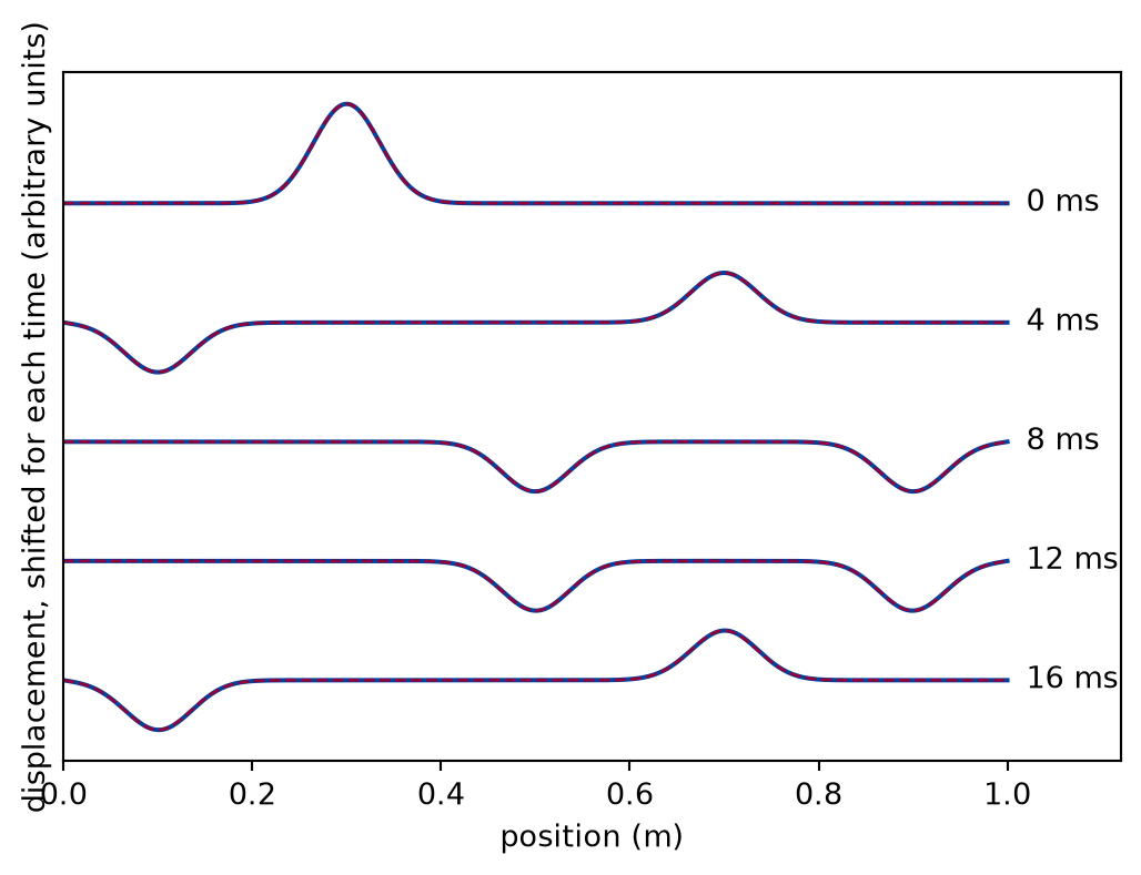
The string is 1 m long, the wave speed is 100 m/s, and it is plucked into a Gaussian bump of width 0.05 m centred at 0.3 m, at rest. Both ends are fixed. The grid has four hundred cells and the Courant number is one half.

LENGTH = 1.0  # string length, m
SPEED = 100.0  # wave speed, m/s

src/pbc/waves/experiments/wave_equation.py, lines 31 to 32, read from the repository when this page was built.

def bump(s):
    return np.exp(-(((s - 0.3) / 0.05) ** 2))

src/pbc/waves/experiments/wave_equation.py, lines 36 to 37, read from the repository when this page was built.

cells = 400
dx = LENGTH / cells
dt = 0.5 * dx / SPEED
x = grid(LENGTH, cells)
snapshot_times = [0.0, 0.004, 0.008, 0.012, 0.016]
steps = round(snapshot_times[-1] / dt)

src/pbc/waves/experiments/wave_equation.py, lines 41 to 46, read from the repository when this page was built.

def pulse_run():
    """The pulse released from rest and its reflections, against the exact
    solution at five times."""
    pulse = solve(
        bump(x), np.zeros_like(x), c=SPEED, dx=dx, dt=dt, n_steps=steps, every=1
    )
    pick = [int(np.argmin(np.abs(pulse.t - t))) for t in snapshot_times]
    exact = [
        reflected_pulse(bump, x, pulse.t[j], length=LENGTH, c=SPEED, ends="fixed")
        for j in pick
    ]
    worst = max(error_norm(pulse.u[j], e) for j, e in zip(pick, exact, strict=True))
    assert worst < 0.01, "the computed pulse leaves the exact one"
    return pulse, pick, exact, worst

src/pbc/waves/experiments/wave_equation.py, lines 55 to 68, read from the repository when this page was built.

def draw_pulse_reflections(pulse, pick, exact) -> Figure:
    """The pulse at five times, computed and exact, shifted for each time."""
    fig, ax = plt.subplots(figsize=(6.4, 4.2))
    for row, (j, e) in enumerate(zip(pick, exact, strict=True)):
        offset = -1.2 * row
        ax.plot(x, pulse.u[j] + offset, color="#00429d")
        ax.plot(x, e + offset, color="#93003a", linestyle="--", linewidth=1)
        ax.text(1.02, offset, f"{pulse.t[j] * 1000:.0f} ms", va="center")
    ax.set_xlabel("position (m)")
    ax.set_ylabel("displacement, shifted for each time (arbitrary units)")
    ax.set_yticks([])
    ax.set_xlim(0, 1.12)
    return fig

src/pbc/waves/experiments/wave_equation.py, lines 71 to 83, read from the repository when this page was built.

Five stacked curves of displacement against position along a string from zero to one metre. The top curve is a single bump near the left. Below it the bump has split in two halves that move apart, then the right half reaches the right end and a half of opposite sign, pointing down, appears to come back from it. — Figure 1: simulated The bump splits into two halves that run apart, and the one that reaches the fixed end at the right comes back turned upside down. Solid lines are the computed field at five times, dashed lines the exact solution, which they cover.

Numerically verified (a Gaussian pulse, fixed ends, Courant number one half, four hundred cells): The computed field follows the exact solution of d’Alembert with a mirror image behind the fixed end. The largest difference between the computed and the exact displacement, over the five times shown, is 0.0049 in units of the pulse height. The pulse that arrives at the right end is turned upside down, which the figure shows and the sign of the continuation explains. The data are simulated; the check is the exact solution.

The error falls as the square of the spacing

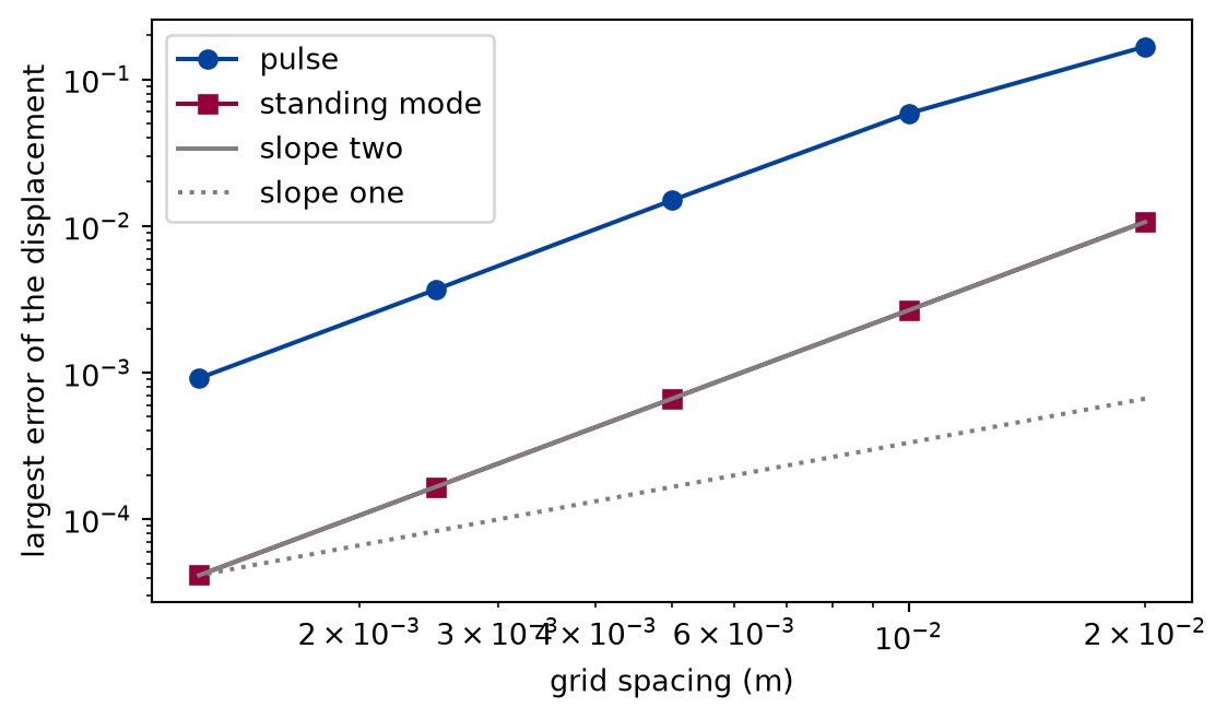
A single picture cannot tell a first-order method from a second-order one. The order is measured: halve the cell, keep the Courant number, compute the same time again, and compare the errors. The time is chosen so that the pulse has been reflected once. The comparison is made for the pulse and for a standing mode, the smooth shape $\sin(3\pi x/L)$ , whose exact solution is a cosine in time.

cell_counts = np.array([50, 100, 200, 400, 800])
pulse_time = 0.012
mode_time = 0.0123

src/pbc/waves/experiments/wave_equation.py, lines 49 to 51, read from the repository when this page was built.

def final_error(n_cells, shape, reference, time):
    h = LENGTH / n_cells
    xs = grid(LENGTH, n_cells)
    n_steps = round(time / (0.5 * h / SPEED))
    result = solve(
        shape(xs),
        np.zeros_like(xs),
        c=SPEED,
        dx=h,
        dt=0.5 * h / SPEED,
        n_steps=n_steps,
        every=n_steps,
    )
    return error_norm(result.u[-1], reference(xs, result.t[-1]))

src/pbc/waves/experiments/wave_equation.py, lines 86 to 99, read from the repository when this page was built.

def pulse_reference(xs, t):
    return reflected_pulse(bump, xs, t, length=LENGTH, c=SPEED, ends="fixed")

src/pbc/waves/experiments/wave_equation.py, lines 102 to 103, read from the repository when this page was built.

def mode_shape(xs):
    return np.sin(3 * np.pi * xs / LENGTH)

src/pbc/waves/experiments/wave_equation.py, lines 106 to 107, read from the repository when this page was built.

def mode_reference(xs, t):
    return standing_mode(xs, t, length=LENGTH, n=3, c=SPEED)

src/pbc/waves/experiments/wave_equation.py, lines 110 to 111, read from the repository when this page was built.

def convergence(experiment: Experiment):
    """The error of the pulse and of the standing mode as the spacing is
    halved, and the fitted orders; record the table."""
    spacing = LENGTH / cell_counts
    pulse_errors = np.array(
        [final_error(n, bump, pulse_reference, pulse_time) for n in cell_counts]
    )
    mode_errors = np.array(
        [final_error(n, mode_shape, mode_reference, mode_time) for n in cell_counts]
    )
    # The coarsest grid of the pulse resolves its width badly, so the order is
    # fitted on the three finest grids.
    pulse_order = observed_order(spacing[-3:], pulse_errors[-3:])
    mode_order = observed_order(spacing, mode_errors)
    assert abs(pulse_order - 2.0) < 0.1 and abs(mode_order - 2.0) < 0.1

    experiment.table(
        "convergence",
        list(zip(cell_counts, spacing, pulse_errors, mode_errors, strict=True)),
        [
            ("cells", "", "d"),
            ("spacing", "m", ".5f"),
            ("error of the pulse", "", ".5f"),
            ("error of the mode", "", ".5f"),
        ],
        "The largest error of the displacement at a fixed time, for the pulse and "
        "for the standing mode, as the spacing is halved with the Courant number "
        "at one half.",
    )
    return spacing, pulse_errors, mode_errors, pulse_order, mode_order

src/pbc/waves/experiments/wave_equation.py, lines 114 to 143, read from the repository when this page was built.

The largest error of the displacement at a fixed time, for the pulse and for the standing mode, as the spacing is halved with the Courant number at one half.
cells	spacing (m)	error of the pulse	error of the mode
50	0.02000	0.16732	0.01070
100	0.01000	0.05856	0.00266
200	0.00500	0.01498	0.00067
400	0.00250	0.00369	0.00017
800	0.00125	0.00092	0.00004

def draw_convergence(spacing, pulse_errors, mode_errors) -> Figure:
    """The error against the spacing, with slopes one and two."""
    fig, ax = plt.subplots(figsize=(6.4, 3.6))
    ax.loglog(spacing, pulse_errors, "o-", color="#00429d", label="pulse")
    ax.loglog(spacing, mode_errors, "s-", color="#93003a", label="standing mode")
    ax.loglog(
        spacing,
        mode_errors[-1] * (spacing / spacing[-1]) ** 2,
        color="gray",
        label="slope two",
    )
    ax.loglog(
        spacing,
        mode_errors[-1] * (spacing / spacing[-1]),
        color="gray",
        linestyle=":",
        label="slope one",
    )
    ax.set_xlabel("grid spacing (m)")
    ax.set_ylabel("largest error of the displacement")
    ax.legend()
    return fig

src/pbc/waves/experiments/wave_equation.py, lines 146 to 167, read from the repository when this page was built.

Log-log plot of error against grid spacing. Two descending lines of markers, one for the pulse and one for the mode, run parallel to a solid reference line of slope two and fall much faster than a dotted reference line of slope one. — Figure 2: simulated The error of the pulse and of the mode against the spacing, on logarithmic axes. Both fall along a line of slope two; the dotted line shows a slope of one for comparison.

Numerically verified (a pulse and a standing mode, fixed ends, Courant number one half, grids of fifty to eight hundred cells): The error of the scheme falls as the second power of the grid spacing at a fixed Courant number. The fitted order is 2.02 for the pulse, on the three finest grids, and 2.00 for the mode. The pulse at the coarsest grid is still outside the regime where the Taylor expansion holds, because a cell is not small compared with the width of the pulse; the table shows the error of the pulse falling by less than a factor of four there. The check is the exact solution, and the order is a measured one: it is the slope of a fitted line, with the finite range of grids it was fitted on.

The CFL limit

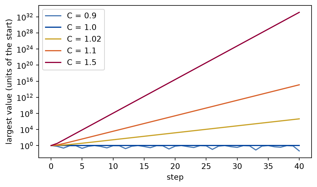
The same program is now run at a Courant number that the stability argument allows and at some that it does not. The starting field is a zigzag of size $10^{-10}$ , which is the size of an error that round-off alone would leave. Everything else is zero. The field is recorded at every step, and the factor by which its largest value grows per step over the last ten steps is compared with the factor of the formula.

courants = [0.5, 0.9, 1.0, 1.02, 1.1, 1.5]

src/pbc/waves/experiments/wave_equation.py, line 171, read from the repository when this page was built.

def cfl_run(experiment: Experiment):
    """A zigzag of the size of round-off at six Courant numbers: its largest
    value and, above the limit, its growth per step; record the table."""
    runs = {c: zigzag_run(c) for c in courants}
    rows = []
    for c in courants:
        result = runs[c]
        peak = np.max(np.abs(result.u))
        if c <= 1.0:
            rows.append((c, peak / 1e-10, None, 1.0))
        else:
            rows.append((c, peak / 1e-10, amplitude_growth(result), growth_factor(c)))
    for _, _, measured, predicted in rows:
        if measured is not None:
            assert abs(measured / predicted - 1.0) < 0.01
    assert all(row[1] < 1.5 for row in rows if row[0] <= 1.0)

    experiment.table(
        "cfl-run",
        rows,
        [
            ("Courant number", "", ".2f"),
            ("largest value over forty steps, in units of the start", "", ".3g"),
            ("measured growth per step", "", ".3f"),
            ("predicted growth per step", "", ".3f"),
        ],
        "The largest value of the field in forty steps from a zigzag of the size of "
        "round-off, and, above the limit, its measured and predicted growth per "
        "step.",
    )
    return runs, rows

src/pbc/waves/experiments/wave_equation.py, lines 175 to 205, read from the repository when this page was built.

The largest value of the field in forty steps from a zigzag of the size of round-off, and, above the limit, its measured and predicted growth per step.
Courant number	largest value over forty steps, in units of the start	measured growth per step	predicted growth per step
0.50	1		1.000
0.90	1		1.000
1.00	1		1.000
1.02	4.33e+06	1.491	1.491
1.10	1.29e+15	2.428	2.428
1.50	1.37e+33	6.854	6.854

def draw_cfl(runs) -> Figure:
    """The largest value of the zigzag against the step, for five Courant
    numbers."""
    fig, ax = plt.subplots(figsize=(6.4, 3.6))
    for c, colour in zip(
        (0.9, 1.0, 1.02, 1.1, 1.5),
        ("#4a7ab5", "#00429d", "#c9a227", "#d9622b", "#93003a"),
        strict=True,
    ):
        size = np.max(np.abs(runs[c].u), axis=1) / 1e-10
        ax.semilogy(size, color=colour, label=f"C = {c}")
    ax.set_xlabel("step")
    ax.set_ylabel("largest value (units of the start)")
    ax.legend()
    return fig

src/pbc/waves/experiments/wave_equation.py, lines 208 to 222, read from the repository when this page was built.

Semi-logarithmic plot of the largest value of the field against the step number, from zero to forty. Lines for the Courant numbers one half and one are flat. Lines for one point zero two, one point one and one point five rise as straight lines, steeper for the larger number, and reach many orders of magnitude above the start. — Figure 3: simulated The largest value of the field at each step, in units of its starting size, for four Courant numbers. Up to one it stays at the level of the start; above one it grows by a fixed factor per step, a straight line on this logarithmic scale.

Numerically verified (a zigzag of size 1e-10, free ends, sixty cells, forty steps): Up to a Courant number of one the field stays at the size of its start; above it the zigzag grows by the factor that the stability calculation predicts. The measured growth per step at the Courant number 1.02 is 1.491 against 1.491 predicted, and at 1.5 it is 6.85 against 6.85. A Courant number only two per cent above the limit multiplies the zigzag by 1.49 at every step, so a start of the size of round-off reaches the size of the pulse after 58 steps. A run past the limit does not degrade gracefully, it ends. At exactly one the scheme has no error at all on the grid: a wave crosses one cell per step, which is what the grid values need to follow it exactly, and the second exercise checks it.

Limits

Only a one-dimensional, linear, lossless, uniform medium. The exact solution exists because of these. A wave in a plane or in space spreads and weakens, a medium that changes reflects, and a nonlinear one steepens its waves into shocks. The scheme still applies with extra terms; the exact checks of this lesson do not.
The order is a property of smooth solutions. A shape with a corner has a larger error than the second-order law says and converges more slowly. The pulse here is smooth and resolved on all but the coarsest grid.
Stability is not accuracy. At a Courant number below one the scheme does not blow up, and still shifts the phase of every wave a little; the next lesson measures that. A scheme that is stable is allowed to be wrong.
The growth rate is that of the shortest mode. The prediction is for the zigzag, which dominates after a few steps. On a run that starts from a smooth shape, the zigzag has to be seeded by round-off first, which takes longer and depends on the machine; the lesson seeds it on purpose.

Self-check. A student halves the cell of a stable run to get a better answer, and keeps the same time step. What happens, and why?

The error halves, because the cell is half as large.

No. The scheme is second order, and the error would fall by a factor of four if the time step were halved as well. With the time step kept, the Courant number changes, and the statement does not follow.
The Courant number doubles. If it was above one half, it is now above one and the run grows without bound.

Correct: the Courant number is the speed times the time step over the cell, so halving the cell doubles it. Refining the grid in space requires a shorter step in time.
Nothing changes, because the scheme is stable.

The scheme is stable only for a Courant number at most one, and the Courant number depends on the cell.

Solution to the self-check

The Courant number is $C = c\,\Delta t/\Delta x$ . With $\Delta t$ kept and $\Delta x$ halved, $C$ doubles. A run at $C = 0.6$ becomes a run at $C = 1.2$ , beyond the limit, and the zigzag grows by a fixed factor at every step. The remedy is to refine in time with the space, which also gives the fourth of the error that second order promises.

Exercises

Exercise 1. A free end. Run the pulse of the first example with both ends free instead of fixed and compare it with the exact solution. Does the reflected pulse come back upright?

Hint 1 of 1 for exercise 1

The solver takes left and right, and the exact solution takes ends.

Solution to exercise 1

def free_ends():
    """Exercise 1: the pulse on a string with free ends; its largest error
    and the part that has returned."""
    free = solve(
        bump(x),
        np.zeros_like(x),
        c=SPEED,
        dx=dx,
        dt=dt,
        n_steps=steps,
        left="free",
        right="free",
        every=steps,
    )
    free_exact = reflected_pulse(
        bump, x, free.t[-1], length=LENGTH, c=SPEED, ends="free"
    )
    free_error = error_norm(free.u[-1], free_exact)
    returned = free.u[-1][x > 0.75]
    return free_error, returned

src/pbc/waves/experiments/wave_equation.py, lines 225 to 244, read from the repository when this page was built.

The largest difference from the exact solution is 0.0049. The part of the field in the right quarter of the string has its largest value 0.17 and its smallest -0.00: it is positive, so it returned upright, as the continuation with the same sign says.

Exercise 2. Exact at the limit. Run the standing mode of the second example at a Courant number of exactly one, on one hundred cells, until the time of the example. How large is the error? Why is it so small?

Hint 1 of 1 for exercise 2

Compare the error with the round-off of double-precision numbers.

Solution to exercise 2

def at_the_limit():
    """Exercise 2: the standing mode at a Courant number of one."""
    n_cells = 100
    h = LENGTH / n_cells
    xs = grid(LENGTH, n_cells)
    at_limit = solve(
        mode_shape(xs),
        np.zeros_like(xs),
        c=SPEED,
        dx=h,
        dt=h / SPEED,
        n_steps=round(mode_time / (h / SPEED)),
        every=round(mode_time / (h / SPEED)),
    )
    return error_norm(at_limit.u[-1], mode_reference(xs, at_limit.t[-1]))

src/pbc/waves/experiments/wave_equation.py, lines 247 to 261, read from the repository when this page was built.

The error is below 1e-12, which is round-off, not method error. At $C = 1$ the two error terms of the scheme, in space and in time, cancel: the scheme moves each value exactly one cell per step, and a wave that is a function of $x - ct$ does the same.

Exercise 3. How much does a zigzag grow? A run at $C = 1.05$ has a zigzag of size $10^{-10}$ . After how many steps has the zigzag grown to the size of a pulse of height one?

Hint 1 of 1 for exercise 3

The growth factor per step comes from the formula of the lesson, and the number of steps from a logarithm.

Solution to exercise 3

def growth_to_one():
    """Exercise 3: the growth per step at a Courant number of 1.05, and the
    steps that bring round-off to one."""
    factor = growth_factor(1.05)
    needed = np.log(1e10) / np.log(factor)
    return factor, needed

src/pbc/waves/experiments/wave_equation.py, lines 264 to 269, read from the repository when this page was built.

The factor is 1.877 per step, so 37 steps bring $10^{-10}$ to one. That is a few dozen steps of a run that would otherwise need thousands; a program above the limit fails within the first fraction of its run.

Run this experiment

This page was built from commit 6417e2ff90258bd2d2ba21d217eb7666fd24f680 of the repository.

In a clone at that commit, with the project’s Python packages installed, this command runs the experiment of this page:

uv run --locked --no-dev python -m pbc.waves.experiments.wave_equation results

Files, tests, and every command

The files behind it:

site/lessons/waves/01-the-wave-equation/index.qmd: this page, with every code cell.
src/pbc/waves/wave.py: code the experiment runs.
src/pbc/waves/experiments/wave_equation.py: code the experiment runs.
src/pbc/experiment.py: code the experiment runs.
tests/unit/test_waves.py: tests of that code.
tests/unit/test_wave_equation_experiment.py: tests of that code.

With Git and uv installed (see the setup page), run:

git clone https://github.com/taspinar/physics-by-construction.git
cd physics-by-construction
git checkout 6417e2ff90258bd2d2ba21d217eb7666fd24f680
uv sync --locked --no-dev
uv run --locked --no-dev python -m pbc.waves.experiments.wave_equation results

The experiment writes every figure of this page into results/, as <label>.png, and every number and table of the page, as the page shows it, into results/results.json. Its numbers match this page to the digits shown, and its figure files are the ones the page shows; digits beyond those can differ between machines, because floating-point libraries differ. Change the code of the experiment and run it again to see what changes.