Equations from noisy trajectories: where differentiation fails

The same equation discovery with measurement noise on the positions: how numerical differentiation amplifies noise, how a smoothing differentiator trades it for bias, and at which noise each way stops recovering the equation, reproducibly over seeded copies.

Course

Classical mechanics, lesson 27 of 31

Methods

Simulation

Difficulty

Advanced, level 3 of 3

What you’ll learn

• Explain why a second difference divides the noise of the positions by the square of the time step, and find the step that balances noise against truncation
• Compare central differences with a Savitzky-Golay filter on the same noisy data, and state the noise at which each stops recovering the equation
• Choose the window of a smoothing filter by the bias it adds on clean data and the noise it removes
• Report a failure of a discovery method as a result, with the evidence of where and why it fails

Prerequisites

Discovering differential equations from trajectories.

Before you begin

• Statistics: the standard deviation of a sum of independent errors

Related

none

Previous

Discovering differential equations from trajectories

Next

Particles in a box

With scripts, this page keeps a record in your browser of whether you completed the lesson. Nothing is stored without them.

With scripts, this place suggests what to do next, with the reason, from the progress saved in your browser. Without them, follow the learning path.

The previous lesson read the equation of a damped oscillator from its positions. The positions were exact. A camera, a laser tracker, or an encoder gives positions with errors, and those errors are small compared with the motion: a millimetre on a swing of a metre. It seems that such small errors should barely matter.

They matter a great deal, because the equation is about the acceleration, and the acceleration is a second derivative. Differentiating measured data is the classical ill-posed step of equation discovery. This lesson measures how ill-posed, compares two ways to differentiate, and records where each fails. The owner’s rule for the lesson is that a failure is a result: the page does not tune a setting until something succeeds, it shows reproducibly, over seeded copies of the noise, at what noise level each method breaks, and why.

Assumptions

1. The system and the regression are those of the previous lesson. The damped oscillator, its four orbits sampled every hundredth of a second, the cubic library, the threshold, and the tolerance of five percent on each coefficient are unchanged.
2. The noise is Gaussian, independent between samples, and the same for every position. Real trackers have correlated errors, outliers, and quantisation; each of these behaves differently under differentiation.
3. Nothing is known about the noise when differentiating. Neither method uses the noise level; the threshold of the regression is the same at every level.
4. The verdict is per noisy copy. At each noise level ten copies of the noise are drawn with fixed seeds, and the page counts in how many the regression keeps exactly the true terms within the tolerance. A count is reproducible; it is not a probability with an error bar.
5. The positions are what is noisy. The library terms are evaluated at the estimated position and velocity, so the noise enters both sides of the regression.

OMEGA2 = 4.0  # k / m, 1/s²
DAMPING = 0.3  # b / m, 1/s
DT = 0.01  # s, the sampling interval
DURATION = 10.0  # s
STARTS = ((1.0, 0.0), (0.0, 2.0), (-0.5, 1.0), (2.0, -1.0))  # x0 (m), v0 (m/s)

src/pbc/mechanics/experiments/discovering_differential_equations.py, lines 37 to 41, read from the repository when this page was built.

Two ways to differentiate

Noise against truncation

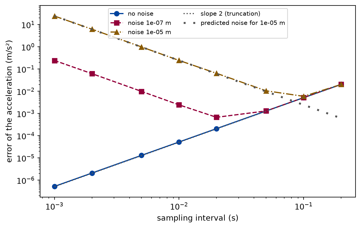
A central second difference adds three positions with weights $1, -2, 1$ and divides by $\Delta t^2$. If each position carries an independent error of standard deviation $\sigma$, the error of the sum has the standard deviation $\sigma\sqrt{1 + 4 + 1} = \sqrt 6\,\sigma$, so the acceleration has a noise of $$\sqrt 6\,\frac{\sigma}{\Delta t^2}.$$ The truncation error, from the Taylor expansion, is $\tfrac{1}{12}\Delta t^2\,x^{(4)}$. Shrinking the step reduces the second and increases the first. With noise there is a best step, and below it the estimate gets worse the finer the sampling.

FINE = 0.001  # s, the step of the reference simulation
STRIDES = (1, 2, 5, 10, 20, 50, 100, 200)  # sampling intervals, in fine steps
STEP_NOISE = (0.0, 1e-7, 1e-5)  # m

src/pbc/mechanics/experiments/equations_from_noisy_trajectories.py, lines 55 to 57, read from the repository when this page was built.

def step_errors() -> dict[float, list[float]]:
    """The root-mean-square error (m/s²) of the central second difference
    against the true acceleration, for each sampling interval and noise."""
    x, v = sampled(*STARTS[0], FINE)
    errors = {}
    for noise in STEP_NOISE:
        rng = np.random.default_rng(5)
        measured = noisy(x, noise, rng)
        errors[noise] = []
        for stride in STRIDES:
            dt = stride * FINE
            data = central_differences(measured[::stride], dt)
            truth = damped(x[::stride][1:-1], v[::stride][1:-1])
            errors[noise].append(float(np.sqrt(((data.a - truth) ** 2).mean())))
    return errors

src/pbc/mechanics/experiments/equations_from_noisy_trajectories.py, lines 84 to 98, read from the repository when this page was built.

def draw_step_errors(errors: dict[float, list[float]]) -> Figure:
    """Log-log error of the second difference against the step, one curve
    per noise, with the slope of truncation and the predicted noise of the
    noisiest record as references."""
    fig, ax = plt.subplots(figsize=(6.4, 4.0), constrained_layout=True)
    steps = np.array(STRIDES) * FINE
    styles = [("o", "-", 0), ("s", "--", 1), ("^", "-.", 3)]
    for (noise, error), (marker, line, colour) in zip(
        errors.items(), styles, strict=True
    ):
        ax.loglog(
            steps,
            error,
            marker=marker,
            linestyle=line,
            color=FIGURE_COLOURS[colour],
            label="no noise" if noise == 0 else f"noise {noise:g} m",
        )
    clean = errors[0.0]
    ax.loglog(
        steps,
        clean[-1] * (steps / steps[-1]) ** 2,
        color=FIGURE_COLOURS[2],
        linestyle=":",
        label="slope 2 (truncation)",
    )
    top = max(errors)
    ax.loglog(
        steps,
        np.sqrt(6) * top / steps**2,
        color=FIGURE_COLOURS[2],
        linestyle=(0, (1, 4)),
        linewidth=2.5,
        label=f"predicted noise for {top:g} m",
    )
    ax.set_ylim(min(clean) / 3, max(max(e) for e in errors.values()) * 3)
    ax.set_xlabel("sampling interval (s)")
    ax.set_ylabel("error of the acceleration (m/s²)")
    ax.legend(loc="upper center", fontsize=8, ncols=2)
    return fig

src/pbc/mechanics/experiments/equations_from_noisy_trajectories.py, lines 101 to 140, read from the repository when this page was built.

Figure 1: simulated Log-log error of the central second difference against the sampling interval, without noise and with two noise levels. Without noise the error falls as the square of the step; with noise it rises as one over the square below a best step, which grows with the noise. The dotted lines are the slope of truncation and the noise predicted for the noisier record, not fits.

The sampling interval with the smallest error of the acceleration for each noise, and that error to two significant digits.

noise (m)	best sampling interval (s)	its error (m/s²)
0	0.001	5.2e-07
1e-07	0.02	6.8e-04
1e-05	0.1	5.9e-03

The best step of a noisy record is far coarser than the sampling interval of the lesson, and even there the error is large compared with a clean record. A fixed recording cannot choose its step freely, so the remedy is to estimate the derivative from more than three samples.

Smoothing: a polynomial over a window

A Savitzky-Golay filter fits a polynomial, here of degree three, by least squares to the samples in a window around each point, and differentiates the polynomial. Over a window of $w$ samples the noise of the derivative shrinks roughly as a power of $w$, because many samples are averaged. The price is a bias: whatever of the motion is not a cubic over the window is smoothed away, and the bias grows with the window.

def savitzky_golay(x: Array, dt: float, window: int, order: int = 3) -> Derivatives:
    """The position, velocity, and acceleration of a polynomial of degree
    ``order`` fitted by least squares to the ``window`` samples around each
    sample of ``x`` (m), sampled every ``dt`` (s). The samples closer than
    half a window to either end are dropped: there the window is one-sided.

    The fit averages the noise over the window and follows any part of the
    motion that is a polynomial of degree ``order`` over it; what is not, it
    smooths away, so the estimate has a bias that grows with the window."""
    x = np.asarray(x, dtype=float)
    if window % 2 == 0 or window <= order:
        raise ValueError(f"the window must be odd and larger than {order}")
    half = window // 2
    inner = slice(half, len(x) - half)

    def derivative(n: int) -> Array:
        return savgol_filter(x, window, order, deriv=n, delta=dt)[inner]

    return Derivatives(derivative(0), derivative(1), derivative(2))

src/pbc/discovery/equations.py, lines 59 to 77, read from the repository when this page was built.

The program

The comparison runs the regression of the previous lesson on noisy copies of the four orbits, once for each differentiator, and counts the copies in which it recovers the equation.

NOISE_LEVELS = (1e-5, 1e-4, 3e-4, 1e-3, 3e-3, 1e-2, 3e-2, 1e-1)  # m
SEEDS = 10
WINDOW = 41  # samples: 0.4 s at the sampling interval of 0.01 s
ORDER = 3  # the degree of the polynomial in the window

src/pbc/mechanics/experiments/equations_from_noisy_trajectories.py, lines 49 to 52, read from the repository when this page was built.

def trials(differentiate: Differentiator, noise: float, dt: float = DT) -> list[bool]:
    """Whether the regression recovers the equation, for each seed."""
    return [recovered(e) for e in fits(differentiate, noise, dt)]

src/pbc/mechanics/experiments/equations_from_noisy_trajectories.py, lines 166 to 168, read from the repository when this page was built.

Worked examples

Recovery against noise

def sweep(
    experiment: Experiment,
) -> tuple[dict[str, list[int]], dict[str, list[float]]]:
    """Recoveries and the median coefficient error of both differentiators at
    every noise level; record the table."""
    counts: dict[str, list[int]] = {}
    errors: dict[str, list[float]] = {}
    for name, d in differentiators().items():
        found = [fits(d, noise) for noise in NOISE_LEVELS]
        counts[name] = [sum(recovered(e) for e in f) for f in found]
        errors[name] = [
            float(np.median([coefficient_error(e) for e in f])) for f in found
        ]
    experiment.table(
        "sweep",
        [
            (
                noise,
                *(counts[name][i] for name in counts),
                *(errors[name][i] for name in errors),
            )
            for i, noise in enumerate(NOISE_LEVELS)
        ],
        columns=[
            ("noise", "m", "g"),
            (f"central differences (of {SEEDS})", "", "d"),
            (f"Savitzky-Golay (of {SEEDS})", "", "d"),
            ("central differences, median error", "", ".1e"),
            ("Savitzky-Golay, median error", "", ".1e"),
        ],
        caption=f"How often the regression recovers the equation from {SEEDS}"
        " noisy copies of the four orbits, at each noise of the positions, and"
        " the median over the copies of the largest relative error of a"
        " coefficient of the true equation (one when a term is dropped).",
    )
    return counts, errors

src/pbc/mechanics/experiments/equations_from_noisy_trajectories.py, lines 177 to 212, read from the repository when this page was built.

How often the regression recovers the equation from 10 noisy copies of the four orbits, at each noise of the positions, and the median over the copies of the largest relative error of a coefficient of the true equation (one when a term is dropped).

noise (m)	central differences (of 10)	Savitzky-Golay (of 10)	central differences, median error	Savitzky-Golay, median error
1e-05	10	10	2.0e-04	2.3e-02
0.0001	10	10	1.9e-03	2.3e-02
0.0003	10	10	6.2e-03	2.3e-02
0.001	0	10	1.0e+00	2.3e-02
0.003	0	10	1.0e+00	2.4e-02
0.01	0	10	2.0e+00	2.6e-02
0.03	0	10	2.4e+01	3.7e-02
0.1	0	0	2.6e+02	1.3e-01

def draw_sweep(counts: dict[str, list[int]], errors: dict[str, list[float]]) -> Figure:
    """The fraction of copies recovered and the median coefficient error
    against the noise, for both differentiators, with the tolerance."""
    fig, (top, bottom) = plt.subplots(
        2, 1, figsize=(6.4, 5.6), sharex=True, constrained_layout=True
    )
    styles = list(zip(("o", "s"), ("-", "--"), FIGURE_COLOURS, strict=False))
    for name, (marker, line, colour) in zip(counts, styles, strict=False):
        style = {"marker": marker, "linestyle": line, "color": colour, "label": name}
        top.semilogx(NOISE_LEVELS, np.array(counts[name]) / SEEDS, **style)
        bottom.loglog(NOISE_LEVELS, errors[name], **style)
    bottom.axhline(TOLERANCE, color="0.3", linestyle=":", label="tolerance")
    top.set_ylabel(f"fraction of {SEEDS} copies recovered")
    top.set_ylim(-0.05, 1.05)
    top.legend(loc="lower left", fontsize=8)
    bottom.set_xlabel("noise of the positions (m)")
    bottom.set_ylabel("median coefficient error (relative)")
    bottom.legend(loc="lower right", fontsize=8)
    return fig

src/pbc/mechanics/experiments/equations_from_noisy_trajectories.py, lines 215 to 233, read from the repository when this page was built.

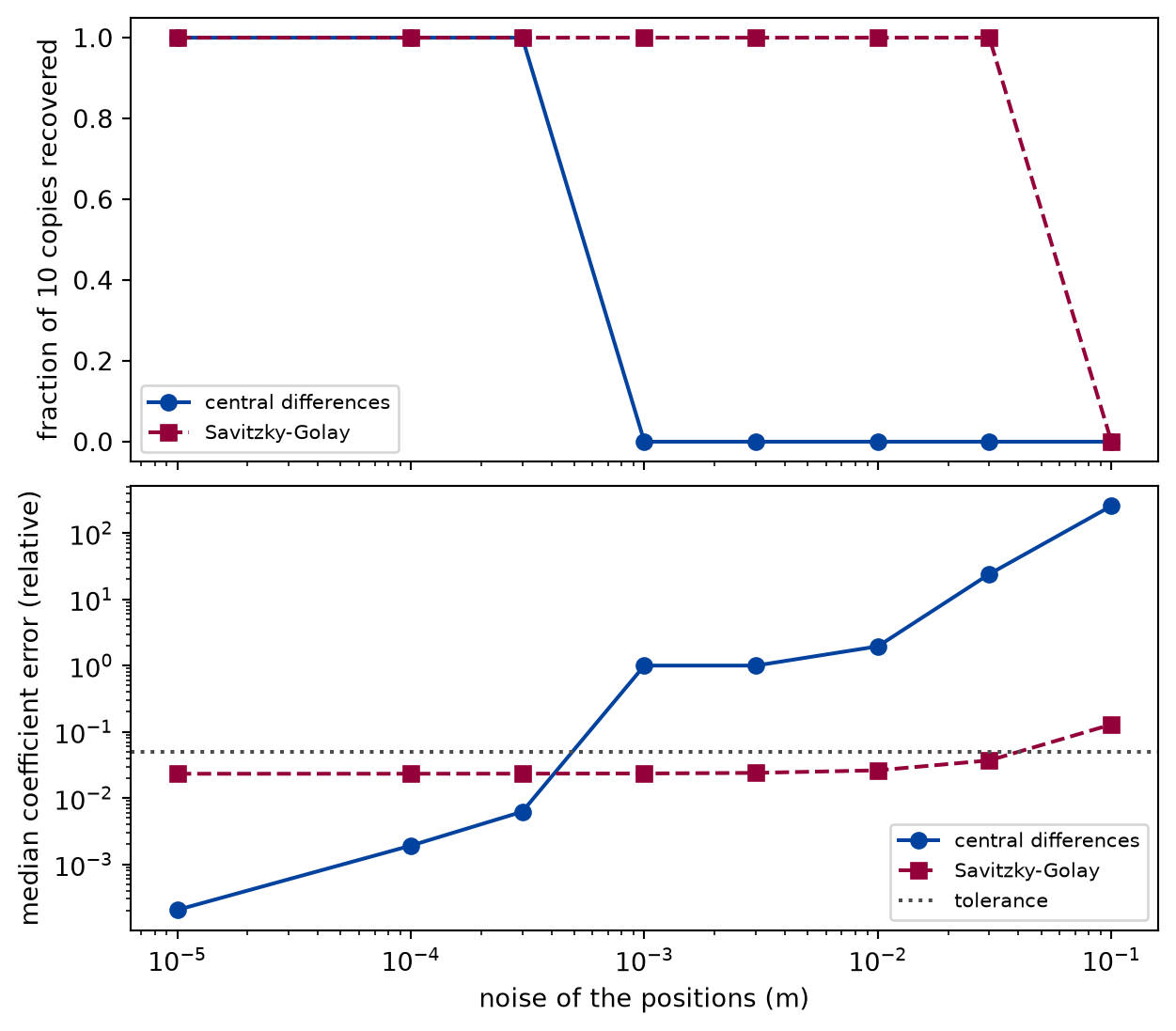
Figure 2: simulated Above, the fraction of noisy copies from which the regression recovers the equation, against the noise of the positions. Below, the median over the copies of the largest relative error of a coefficient, with the tolerance as a dotted line. Central differences fail at a far smaller noise than the Savitzky-Golay filter, and both fail at the largest noise.

Numerically verified (the damped oscillator of the previous lesson, four orbits sampled every 0.01 s, ten seeded copies per noise level, tolerance of five percent): With central differences the regression recovers the equation from every copy up to a noise of 0.0003 m, and from none at 0.001 m and above. With the Savitzky-Golay filter of 41 samples it recovers it from every copy up to 0.03 m.

The lower panel shows how the estimates degrade before the equation is lost. The error of central differences grows with the noise from the smallest level and passes the tolerance between 0.0003 m and 0.001 m. The error of the filter starts higher, at the bias of its window (2.3 percent on clean data, see the window table below), and stays under the tolerance until the largest noise.

Why central differences fail. At a noise of 0.001 m the second difference has a noise of about 24 $\mathrm{m/s^2}$, while the acceleration itself has a root-mean-square of 1.6 $\mathrm{m/s^2}$ on the first orbit. The signal is buried, and the least squares fit attributes the noise to whichever term it correlates with: the damping term, the smallest, is lost first.

Why the filter works, and why it fails too. The window of 0.4 s averages the noise of many samples, so the derivatives stay usable at much larger noise. At the largest noise, 0.1 m, it finds a = -4.23 x - 0.295 v + 0.142 x^3 from the first copy, with a spurious cubic term. The remaining noise in the smoothed velocity and position enters the library columns as well as the target, and the regression mistakes it for structure.

The window: bias against noise

def windows(experiment: Experiment) -> None:
    """Recoveries of the Savitzky-Golay filter for each window and noise;
    record the table."""
    rows = []
    for window in WINDOWS:
        d = differentiators(window)["Savitzky-Golay"]
        rows.append(
            (window, window * DT, *(sum(trials(d, noise)) for noise in WINDOW_NOISE))
        )
    experiment.table(
        "windows",
        rows,
        columns=[
            ("window", "samples", "d"),
            ("window", "s", ".2f"),
            *((f"noise {noise:g} m", "", "d") for noise in WINDOW_NOISE),
        ],
        caption=f"How often, of {SEEDS} copies, the Savitzky-Golay filter of each"
        " window leads to the equation, at each noise of the positions.",
    )

src/pbc/mechanics/experiments/equations_from_noisy_trajectories.py, lines 241 to 260, read from the repository when this page was built.

How often, of 10 copies, the Savitzky-Golay filter of each window leads to the equation, at each noise of the positions.

window (samples)	window (s)	noise 0 m	noise 0.001 m	noise 0.01 m	noise 0.03 m	noise 0.1 m
11	0.11	10	10	6	0	0
21	0.21	10	10	10	3	0
41	0.41	10	10	10	10	0
61	0.61	0	0	3	3	1
81	0.81	0	0	0	0	0

def clean_bias(window: int) -> float:
    """The largest relative error of a coefficient found from clean
    positions through the filter of ``window`` samples."""
    terms = polynomial_library(DEGREE)
    d = differentiators(window)["Savitzky-Golay"]
    data = combine([d(sampled(*s, DT)[0], DT) for s in STARTS])
    found = sparse_regression(terms, data).coefficients
    true = {"x": -OMEGA2, "v": damped(0.0, 1.0)}
    return max(abs(found.get(t, 0.0) / c - 1) for t, c in true.items())

src/pbc/mechanics/experiments/equations_from_noisy_trajectories.py, lines 263 to 271, read from the repository when this page was built.

Numerically verified (the damped oscillator, cubic filter, ten seeded copies per cell): The window that tolerates the most noise is not the widest. On clean positions the filter of 41 samples biases a coefficient by 2.3 percent, within the tolerance, and the filter of 61 samples by 5.1 percent, beyond it, so the wide windows fail even without noise, while the narrow ones fail at lower noise. There is no window that works for every noise level, and the best one depends on the time scale of the motion: the window must be short against the period for the cubic to follow the oscillation, and long against the sampling interval to average the noise. Choosing it by trying windows until the expected equation appears would be choosing the answer; here the window was fixed before the sweep, and the table shows what the others would have done.

Limits

• One system, one library, one threshold. The noise levels at which the methods fail are properties of this oscillator, sampled this way, with this regression. A faster motion, a longer record, or a different threshold moves them.
• Counts over ten seeds are coarse. A level where five of ten copies succeed is a transition, not a measured probability. More seeds would narrow it; the seeds are fixed so that the counts are reproducible.
• The noise is white and known only to the simulation. Correlated noise, outliers, or a quantised encoder change the picture; a filter tuned for one can fail on another.
• Other remedies exist and are not tested here. Fitting splines, regularised differentiation, or the weak formulation (integrating the equation against test functions instead of differentiating the data) can tolerate more noise. They also have settings, and the same rule applies: fix them before looking at the result.
• Recovered means the terms and the tolerance. A copy counts as a success only with exactly the true terms within five percent. A copy that fails this test may still predict the motion well; prediction is a different question, and the previous lesson’s held-out test is the way to ask it.

In plain words: differentiation turns small errors in positions into large errors in accelerations. Smoothing helps by orders of magnitude and adds a bias of its own, and at enough noise every method in this lesson fails. That level, and the reason, are results worth stating.

Self-check. A colleague doubles the sampling rate of the tracker to get better accelerations from central differences, with the same noise per position. What happens to the noise of the second difference?

1. It halves, because there are twice as many samples.

   Each second difference uses only three neighbouring samples; more samples elsewhere do not average its noise.

2. It grows fourfold, because the noise is divided by the square of the step.

   Right. Halving the step multiplies $\sqrt 6\,\sigma/\Delta t^2$ by four, while the truncation error falls by four, which matters only if it was the larger error.

3. It stays the same, because the noise per position is the same.

   The noise per position is the same, but the difference divides it by a smaller step.

Solution to the self-check

It grows by a factor of four: the noise of a central second difference is $\sqrt 6\,\sigma/\Delta t^2$. Faster sampling helps only a method that averages over a fixed duration, like the filter with a window of the same length in seconds.

Exercises

Exercise 1. Sample twice as fast. Halve the sampling interval to 0.005 s, keep the noise per position, and keep the filter’s window at 0.4 s, which is now 81 samples. Count the recoveries of both methods at noise levels of 0.0003, 0.03, and 0.1 m.

Hint 1 of 1 for exercise 1

Central differences use three samples whatever the rate. How many samples does the filter now average over in its window?

Solution to exercise 1

def finer_sampling(experiment: Experiment) -> None:
    """Exercise: half the sampling interval, with the window of the filter
    kept at the same duration."""
    dt = DT / 2
    rows = []
    for noise in (3e-4, 3e-2, 1e-1):
        rows.append(
            (
                noise,
                sum(trials(central_differences, noise)),
                sum(trials(central_differences, noise, dt)),
                sum(trials(differentiators(WINDOW)["Savitzky-Golay"], noise)),
                sum(
                    trials(differentiators(2 * WINDOW - 1)["Savitzky-Golay"], noise, dt)
                ),
            )
        )
    experiment.table(
        "finer-sampling",
        rows,
        columns=[
            ("noise", "m", "g"),
            ("central, 0.01 s", "", "d"),
            ("central, 0.005 s", "", "d"),
            ("filter, 0.01 s", "", "d"),
            ("filter, 0.005 s", "", "d"),
        ],
        caption=f"Recoveries, of {SEEDS} copies, at the sampling interval of the"
        " lesson and at half of it; the filter keeps a window of 0.4 s.",
    )

src/pbc/mechanics/experiments/equations_from_noisy_trajectories.py, lines 281 to 310, read from the repository when this page was built.

Recoveries, of 10 copies, at the sampling interval of the lesson and at half of it; the filter keeps a window of 0.4 s.

noise (m)	central, 0.01 s	central, 0.005 s	filter, 0.01 s	filter, 0.005 s
0.0003	10	0	10	10
0.03	0	0	10	10
0.1	0	0	0	3

Central differences lose the equation at a noise they handled before: the step is halved, so the noise of the acceleration is four times larger. The filter, averaging twice as many samples over the same duration, does as well or better, and recovers some copies at the largest noise. More data help a method only if the method uses them.

Run this experiment

This page was built from commit 3a83ab640162bf2b624c2b254d917ed5bdc7090d of the repository.

In a clone at that commit, with the project’s Python packages installed, this command runs the experiment of this page:

uv run --locked --no-dev python -m pbc.mechanics.experiments.equations_from_noisy_trajectories results

Files, tests, and every command

The files behind it:

• site/lessons/agents-llm/10-equations-from-noisy-trajectories/index.qmd: this page, with every code cell.
• src/pbc/discovery/equations.py: code the experiment runs.
• src/pbc/mechanics/integrators.py: code the experiment runs.
• src/pbc/mechanics/experiments/discovering_differential_equations.py: code the experiment runs.
• src/pbc/mechanics/experiments/equations_from_noisy_trajectories.py: code the experiment runs.
• src/pbc/experiment.py: code the experiment runs.
• tests/unit/test_equations.py: tests of that code.
• tests/unit/test_equations_from_noisy_trajectories_experiment.py: tests of that code.

With Git and uv installed (see the setup page), run:

git clone https://github.com/taspinar/physics-by-construction.git
cd physics-by-construction
git checkout 3a83ab640162bf2b624c2b254d917ed5bdc7090d
uv sync --locked --no-dev
uv run --locked --no-dev python -m pbc.mechanics.experiments.equations_from_noisy_trajectories results

The experiment writes every figure of this page into results/, as <label>.png, and every number and table of the page, as the page shows it, into results/results.json. Its numbers match this page to the digits shown, and its figure files are the ones the page shows; digits beyond those can differ between machines, because floating-point libraries differ. Change the code of the experiment and run it again to see what changes.