Discovering differential equations from trajectories

The equation of motion of a damped oscillator recovered from positions alone, with numerical derivatives and a sparse regression over a library of terms, tested from a start it never saw, and the cases where the data or the library cannot settle the equation.

Course

Classical mechanics, lesson 23 of 31

Slot

D8, number 8 of the 13 slots of the path Scientific law discovery

Methods

Simulation

Difficulty

Advanced, level 3 of 3

What you’ll learn

Estimate velocity and acceleration from sampled positions with central differences, and state their error
Find an equation of motion as a sparse sum of library terms with sequentially thresholded least squares
Test a found equation by integrating it from a held-out start
Detect with the singular values of the library when the data admit several equations, and say which data remove the ambiguity

Prerequisites

The harmonic oscillator, Numerical integrators, Symbolic regression: a law from simulated data.

Before you begin

Calculus: derivatives and the Taylor expansion to fourth order
Linear algebra: least squares and the singular values of a matrix

Previous

Symbolic regression: a law from simulated data

Next

Equations from noisy trajectories: where differentiation fails

With scripts, this page keeps a record in your browser of whether you completed the lesson. Nothing is stored without them.

With scripts, this place suggests what to do next, with the reason, from the progress saved in your browser. Without them, follow the learning path.

The previous lesson found a formula for one number, the period. Mechanics is mostly not about such numbers: it is about equations of motion, the rule that gives the acceleration from the state. Newton wrote them down from principles. A camera that tracks a mass on a spring records something else, a list of positions at equal times. Can the equation be read back from that list?

The approach of this lesson, known as sparse identification of nonlinear dynamics, has two steps. First the derivatives that the equation is about, velocity and acceleration, are estimated from the positions. Then the acceleration is written as a combination of a few terms out of a large library of candidates, $1, x, v, x^2, xv, \dots$ , keeping only those the data need. The result is an equation a person can read, and that can be integrated from any start to test it.

The lesson uses clean data: the positions are exact up to the simulation. The next lesson adds measurement noise, which is where this approach meets its hardest problem. No language model is used.

Assumptions

The positions come from a simulation and are sampled without noise. A damped oscillator, $\ddot x = -\omega^2 x - b\,\dot x$ , is integrated with the fourth-order Runge-Kutta method and sampled every hundredth of a second. Only the positions are kept. With noise, the derivatives degrade; that is the next lesson.
The equation is autonomous and of second order. The acceleration is a function of the position and the velocity, not of time. A driven oscillator would need time in the library.
The law is a sum of the library’s terms. The library holds every product $x^i v^j$ with $i + j \le 3$ . A law that is not such a sum, like the $\sin x$ of a pendulum, can only be approximated; the exercise shows what that means.
Small terms are dropped by a stated rule. A term whose contribution to the acceleration is below two percent of the root-mean-square acceleration is removed. A real term smaller than that is lost; a spurious term larger than that is kept.
The trajectories decide what can be told apart. Four orbits from different starts are used. What one orbit cannot distinguish is shown in the worked examples.

From positions to an equation

Derivatives from samples

With positions $x_k$ every $\Delta t$ , the central differences $v_k \approx \frac{x_{k+1} - x_{k-1}}{2\Delta t}, \qquad a_k \approx \frac{x_{k+1} - 2x_k + x_{k-1}}{\Delta t^2}$ follow from the Taylor expansion of $x(t \pm \Delta t)$ : the odd terms cancel in the first, the even ones in the second, and what is left is an error proportional to $\Delta t^2$ . For a motion of angular frequency $\omega$ , the relative error of the acceleration is about $(\omega\Delta t)^2/12$ , here far below the tolerance.

def central_differences(x: Array, dt: float) -> Derivatives:
    """The velocity ``(x[i+1] - x[i-1]) / (2 dt)`` and the acceleration
    ``(x[i+1] - 2 x[i] + x[i-1]) / dt**2`` at every interior sample of the
    positions ``x`` (m), sampled every ``dt`` (s). Both are second order in
    ``dt``; a noise of standard deviation ``s`` in ``x`` becomes a noise of
    about ``s / dt`` in the velocity and ``2.4 s / dt**2`` in the acceleration.
    """
    x = np.asarray(x, dtype=float)
    return Derivatives(
        x=x[1:-1],
        v=(x[2:] - x[:-2]) / (2 * dt),
        a=(x[2:] - 2 * x[1:-1] + x[:-2]) / dt**2,
    )

src/pbc/discovery/equations.py, lines 44 to 56, read from the repository when this page was built.

A sparse sum of library terms

Every sample gives one equation: the acceleration estimate equals the sum of the library terms, evaluated at that sample’s position and velocity, times unknown coefficients. Thousands of samples and ten terms make an overdetermined linear system, solved by least squares. Least squares alone would give every term a small coefficient, because the derivative errors leak into all of them. Sequentially thresholded least squares removes the terms whose contribution is below the threshold and fits the rest again, until nothing changes.

def sparse_regression(
    terms: Sequence[str], data: Derivatives, threshold: float = THRESHOLD
) -> Equation:
    """Sequentially thresholded least squares: fit the acceleration with all
    ``terms``, drop each term whose contribution is below ``threshold`` times
    the root-mean-square acceleration, and fit the rest again, until no term
    is dropped."""
    columns = evaluate(terms, data.x, data.v)
    scale = np.sqrt((columns**2).mean(axis=0))
    scale[scale == 0] = 1.0
    scaled = columns / scale
    target = data.a
    size = np.sqrt((target**2).mean())
    active = np.ones(len(terms), dtype=bool)
    fitted = np.zeros(len(terms))
    for _ in range(len(terms)):
        fitted[:] = 0.0
        fitted[active], *_ = np.linalg.lstsq(scaled[:, active], target, rcond=None)
        small = active & (np.abs(fitted) < threshold * size)
        if not small.any():
            break
        active &= ~small
    coefficients = fitted / scale
    residual = float(np.sqrt(((target - columns @ coefficients) ** 2).mean()))
    return Equation(
        {t: float(c) for t, c in zip(terms, coefficients, strict=True) if c != 0.0},
        residual,
    )

src/pbc/discovery/equations.py, lines 160 to 187, read from the repository when this page was built.

The damped oscillator

OMEGA2 = 4.0  # k / m, 1/s²
DAMPING = 0.3  # b / m, 1/s
DT = 0.01  # s, the sampling interval
DURATION = 10.0  # s
STARTS = ((1.0, 0.0), (0.0, 2.0), (-0.5, 1.0), (2.0, -1.0))  # x0 (m), v0 (m/s)

src/pbc/mechanics/experiments/discovering_differential_equations.py, lines 37 to 41, read from the repository when this page was built.

DEGREE = 3  # the library: every x^i v^j with i + j <= 3
TOLERANCE = 0.05  # relative, on each coefficient of the true equation
TRUE = {"x": -OMEGA2, "v": -DAMPING}

src/pbc/mechanics/experiments/discovering_differential_equations.py, lines 44 to 46, read from the repository when this page was built.

def discover(experiment: Experiment) -> Equation:
    """Positions of four damped orbits, central differences, and the sparse
    regression; record the coefficients of every term."""
    terms = polynomial_library(DEGREE)
    data = combine([central_differences(positions(damped, *s), DT) for s in STARTS])
    equation = sparse_regression(terms, data)
    experiment.table(
        "coefficients",
        [(t, TRUE.get(t, 0.0), equation.coefficients.get(t)) for t in terms],
        columns=[
            ("term", "", "s"),
            ("true coefficient", "", ".4f"),
            ("found coefficient", "", ".4f"),
        ],
        caption="Each term of the library, its coefficient in the true equation,"
        " and its coefficient in the found one, to four decimals; an empty cell"
        " is a term the regression dropped. The unit of a coefficient is that of"
        " the acceleration divided by that of the term.",
    )
    return equation

src/pbc/mechanics/experiments/discovering_differential_equations.py, lines 93 to 112, read from the repository when this page was built.

Each term of the library, its coefficient in the true equation, and its coefficient in the found one, to four decimals; an empty cell is a term the regression dropped. The unit of a coefficient is that of the acceleration divided by that of the term.
term	true coefficient	found coefficient
1	0.0000
x	-4.0000	-3.9999
v	-0.3000	-0.3000
x^2	0.0000
x v	0.0000
v^2	0.0000
x^3	0.0000
x^2 v	0.0000
x v^2	0.0000
v^3	0.0000

Numerically verified (the simulated damped oscillator, positions without noise every 0.01 s, the cubic library): From the positions of four orbits, 3996 samples in all, the regression over 10 terms finds a = -4 x - 0.3 v: it keeps exactly the two terms of the true equation, and its largest coefficient error is 0.003 percent, within the tolerance of 5 percent. The equation is recovered. The other terms are not merely small: they are absent. That is the point of the threshold. A coefficient of a millionth on $x^3$ would claim a nonlinearity that the oscillator does not have.

The program

The library is generated from its degree, and every term is a product of powers of the position and the velocity. The regression scales each column to a root-mean-square of one before it fits, so that the threshold compares contributions, not coefficients in different units.

def polynomial_library(degree: int = 3) -> tuple[str, ...]:
    """The terms ``x^i v^j`` with ``i + j <= degree``, by degree:
    ``1, x, v, x^2, x v, v^2, ...``."""
    names = []
    for total in range(degree + 1):
        for j in range(total + 1):
            names.append(_term(total - j, j))
    return tuple(names)

src/pbc/discovery/equations.py, lines 89 to 96, read from the repository when this page was built.

def singular_values(terms: Sequence[str], data: Derivatives) -> Array:
    """The singular values of the library on ``data``, each column scaled to a
    root-mean-square of one, relative to the largest. A value near zero is a
    combination of terms that vanishes on the data: the data cannot tell an
    equation from the same equation plus that combination."""
    columns = evaluate(terms, data.x, data.v)
    columns = columns / np.sqrt((columns**2).mean(axis=0))
    values = np.linalg.svd(columns, compute_uv=False)
    return values / values[0]

src/pbc/discovery/equations.py, lines 124 to 132, read from the repository when this page was built.

Worked examples

A start the regression never saw

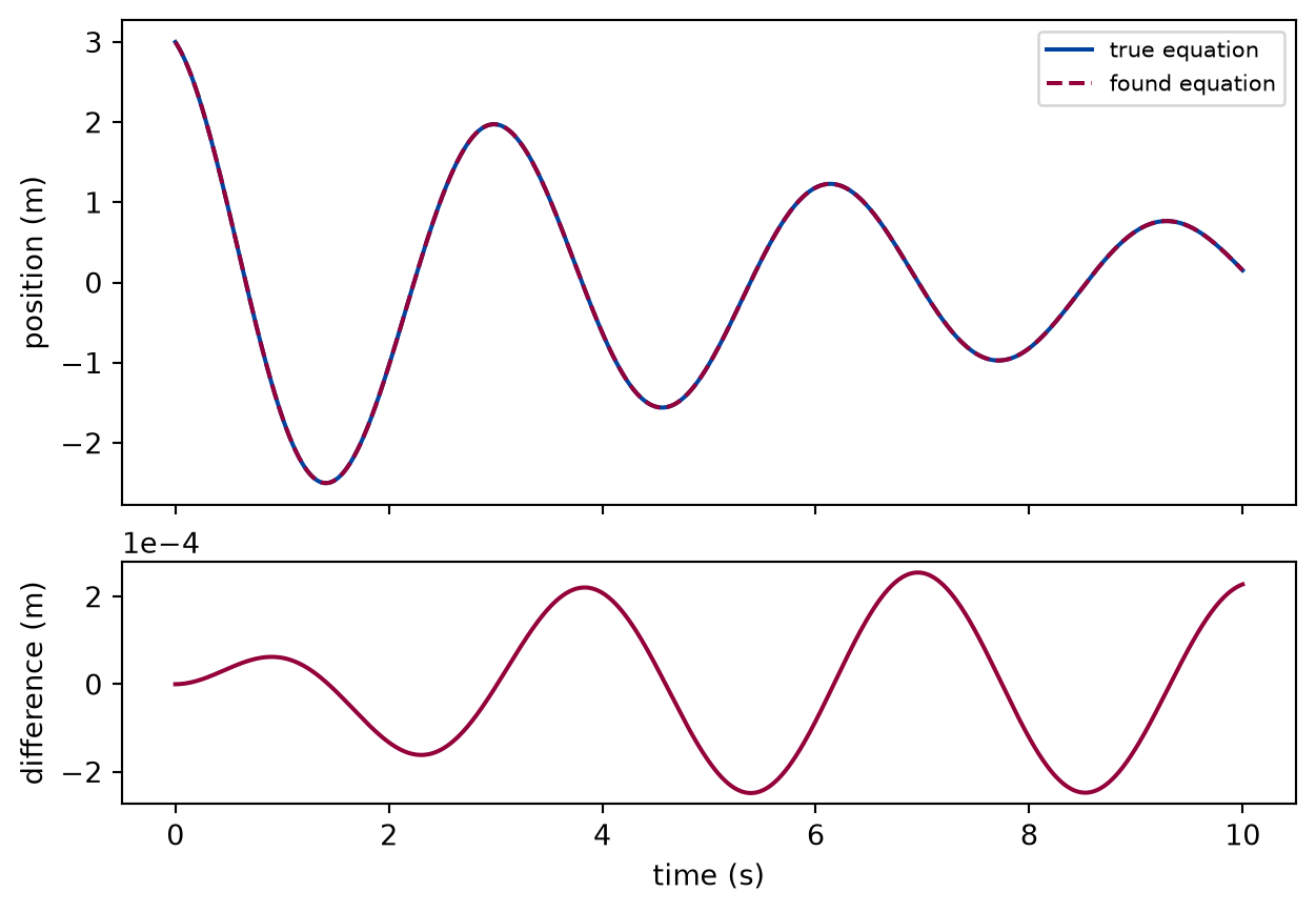
An equation is a claim about every start, not only the four it was read from. The test is to integrate it from a start outside every training orbit and compare with the true motion.

HELD_OUT = (3.0, -2.0)  # x0 (m), v0 (m/s): outside every training orbit

src/pbc/mechanics/experiments/discovering_differential_equations.py, line 49, read from the repository when this page was built.

def held_out(equation: Equation) -> tuple[np.ndarray, np.ndarray, np.ndarray]:
    """The true motion from the held-out start and the motion of the found
    equation from it, over the duration."""
    t = np.arange(round(DURATION / DT) + 1) * DT
    truth = integrate(damped, *HELD_OUT, t)
    found = integrate(equation.acceleration, *HELD_OUT, t)
    return t, truth, found

src/pbc/mechanics/experiments/discovering_differential_equations.py, lines 115 to 121, read from the repository when this page was built.

def draw_held_out(t: np.ndarray, truth: np.ndarray, found: np.ndarray) -> Figure:
    """The true and the found motion from the held-out start, and their
    difference."""
    fig, (top, bottom) = plt.subplots(
        2,
        1,
        figsize=(6.4, 4.4),
        sharex=True,
        constrained_layout=True,
        gridspec_kw={"height_ratios": [2, 1]},
    )
    top.plot(t, truth, color=FIGURE_COLOURS[0], linestyle="-", label="true equation")
    top.plot(t, found, color=FIGURE_COLOURS[1], linestyle="--", label="found equation")
    top.set_ylabel("position (m)")
    top.legend(loc="upper right", fontsize=8)
    bottom.plot(t, found - truth, color=FIGURE_COLOURS[1], linestyle="-")
    bottom.set_ylabel("difference (m)")
    bottom.set_xlabel("time (s)")
    bottom.ticklabel_format(axis="y", style="sci", scilimits=(0, 0))
    return fig

src/pbc/mechanics/experiments/discovering_differential_equations.py, lines 124 to 143, read from the repository when this page was built.

Two panels sharing a time axis from zero to ten seconds. The upper panel shows a decaying oscillation of position; a solid and a dashed curve lie on top of each other. The lower panel shows the difference between them as a small oscillation that grows slowly with time, on an axis scaled by a power of ten. — Figure 1: simulated The motion from a held-out start under the true equation (solid) and under the found one (dashed), and their difference below. The curves coincide over the ten seconds, and the difference stays small against the amplitude.

Numerically verified (one held-out start, ten seconds, the damped oscillator): Integrated from the held-out start, of amplitude 3.0 m, larger than any training orbit, the found equation follows the true motion over ten seconds within 2.5e-04 m. The difference grows slowly because the found coefficients differ slightly from the true ones, and an error of the frequency accumulates as a phase. The test supports the equation over this range of amplitudes and this duration; it says nothing about amplitudes where a real spring stops being linear.

One orbit admits several equations

Now take an oscillator without damping and a single orbit. On that orbit the energy is conserved: $\omega^2 x^2 + v^2$ keeps the value $E$ it started with. So the combination $x\,(\omega^2 x^2 + v^2 - E)$ of library terms is zero at every sample. Add any multiple of it to the true equation and the new equation fits the orbit exactly as well.

ORBIT = (1.0, 0.0)  # x0 (m), v0 (m/s) of the undamped orbit
OTHER_ORBIT = (2.0, 0.0)
LAMBDA = 1.0  # 1/s², the size of the added term

src/pbc/mechanics/experiments/discovering_differential_equations.py, lines 52 to 54, read from the repository when this page was built.

def one_orbit(experiment: Experiment) -> tuple[np.ndarray, np.ndarray]:
    """The library on one orbit and on four orbits of the undamped
    oscillator, and an equation the one orbit cannot tell from the true one;
    record the residual of both on the orbit and on another one."""
    terms = polynomial_library(DEGREE)
    single = central_differences(positions(undamped, *ORBIT), DT)
    several = combine(
        [central_differences(positions(undamped, *s), DT) for s in STARTS]
    )
    # On the orbit the energy per mass, (OMEGA2 x^2 + v^2) / 2, keeps the
    # value it starts with; the added term is zero there and nowhere else.
    energy = OMEGA2 * ORBIT[0] ** 2 + ORBIT[1] ** 2
    true = Equation({"x": -OMEGA2}, 0.0)
    rival = Equation(
        {
            "x": -OMEGA2 - LAMBDA,
            "x^3": LAMBDA * OMEGA2 / energy,
            "x v^2": LAMBDA / energy,
        },
        0.0,
    )
    other = central_differences(positions(undamped, *OTHER_ORBIT), DT)

    def residual(equation: Equation, data) -> float:
        return float(
            np.sqrt(((data.a - equation.acceleration(data.x, data.v)) ** 2).mean())
        )

    experiment.table(
        "rival-equations",
        [
            (equation.formula(), residual(equation, single), residual(equation, other))
            for equation in (true, rival)
        ],
        columns=[
            ("equation", "", "s"),
            ("residual on the orbit", "m/s²", ".2g"),
            ("residual on another orbit", "m/s²", ".2g"),
        ],
        caption="Two equations on the orbit they were read from and on an orbit of"
        " twice the amplitude: the root-mean-square difference between the"
        " acceleration from central differences and the equation's, to two"
        " significant digits.",
    )
    return singular_values(terms, single), singular_values(terms, several)

src/pbc/mechanics/experiments/discovering_differential_equations.py, lines 146 to 190, read from the repository when this page was built.

Two equations on the orbit they were read from and on an orbit of twice the amplitude: the root-mean-square difference between the acceleration from central differences and the equation's, to two significant digits.
equation	residual on the orbit (m/s²)	residual on another orbit (m/s²)
a = -4 x	9.5e-05	0.00019
a = -5 x + 1 x^3 + 0.25 x v^2	0.00012	4.3

The two equations differ by three terms and fit the orbit equally well, to the error of the differences. On an orbit of another energy the added terms no longer vanish, and the rival is far off. The data of one orbit contain no reason to prefer the simpler equation; only the threshold, a rule of the method, does.

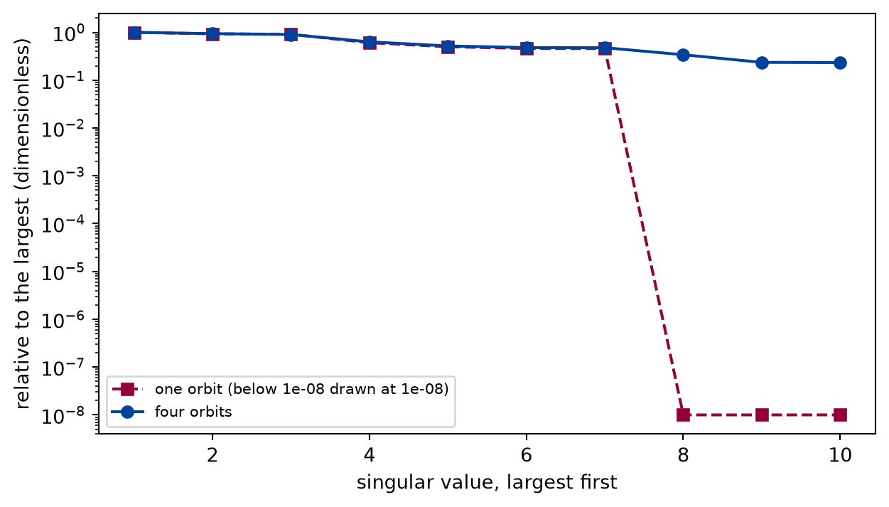
The singular values of the library show the problem without guessing the rival. A singular value near zero is a combination of terms that vanishes on the data: a direction in which the coefficients are not determined.

def draw_singular_values(
    single: np.ndarray, several: np.ndarray, floor: float
) -> Figure:
    """The singular values of the library on one orbit and on four."""
    fig, ax = plt.subplots(figsize=(6.4, 3.6), constrained_layout=True)
    index = np.arange(1, len(single) + 1)
    ax.semilogy(
        index,
        np.maximum(single, floor),
        color=FIGURE_COLOURS[1],
        marker="s",
        linestyle="--",
        label=f"one orbit (below {floor:g} drawn at {floor:g})",
    )
    ax.semilogy(
        index,
        several,
        color=FIGURE_COLOURS[0],
        marker="o",
        linestyle="-",
        label="four orbits",
    )
    ax.set_xlabel("singular value, largest first")
    ax.set_ylabel("relative to the largest (dimensionless)")
    ax.legend(loc="lower left", fontsize=8)
    return fig

src/pbc/mechanics/experiments/discovering_differential_equations.py, lines 193 to 218, read from the repository when this page was built.

Line plot with markers on a logarithmic vertical axis of relative singular value against its rank, largest first. The solid curve for four orbits falls gently and stays within two orders of magnitude of one. The dashed curve for one orbit follows a similar course for its first values and then drops by many orders of magnitude to a flat floor for its last values. — Figure 2: simulated Singular values of the library, relative to the largest, on one orbit and on four orbits of the undamped oscillator. On one orbit several of them collapse, drawn at the floor of the axis: conserved energy ties combinations of terms. Four orbits of different energies remove the ties.

Numerically verified (the undamped oscillator, the cubic library, central differences of exact positions): On one orbit of the undamped oscillator 3 singular values of the library are below 1e-08 of the largest: energy conservation makes $1, x^2, v^2$ dependent, and multiplying the relation by $x$ and by $v$ gives two more. On four orbits the smallest is 0.23, and the equation is determined. This is identifiability in its plainest form. Several formulas describe the same observations whenever the observations satisfy a relation the library can express. A conserved quantity is such a relation, which is a little ironic: the most important property of the motion hides its equation. The remedy is data that break the relation, such as several energies, or a library chosen so that the relation cannot be written in it.

Limits

Clean data only. The derivatives here are exact up to the time step. With measurement noise, the second difference is the weak point; the next lesson measures how weak and compares a smoothing differentiator.
The library is the hypothesis space. The regression can only answer in terms of $x^i v^j$ up to degree three. A law outside it is approximated by a sum that fits the training range and may fail beyond, as the pendulum exercise shows.
The threshold is a choice. Two percent of the acceleration is the stated rule. A real term below it, a weak damping for instance, would be dropped, and nothing in the data would warn.
One held-out start is one test. The found equation agrees with the truth from one start for ten seconds. That supports it over the probed amplitudes, not for every start or every time.
Recovered is not explained. The regression returns coefficients, not their meaning. That the $x$ coefficient is a stiffness over a mass and the $v$ coefficient a damping rate is the reader’s physics, not the method’s output.

In plain words: numerical derivatives and a sparse regression read the equation of a simulated oscillator back from its positions, and the equation holds from a start it never saw. Whether it is the equation depends on whether the data could have told it apart from others, and the singular values of the library are the place to look.

Self-check. A regression on a single long orbit of an undamped oscillator returns $a = -4x$ , the right equation. Why is this not evidence that the data determine the equation?

With scripts, you can record in this browser that you answered this question.

Solution to the self-check

On one orbit the conserved energy makes a combination of library terms vanish, so the true equation plus any multiple of that combination fits equally well. The threshold picked the simplest member of that family; the data did not. Orbits of different energies, or a check of the singular values, are needed before the result is evidence.

Exercises

Exercise 1. A pendulum through a polynomial library. A pendulum with $g/L = 4$ per square second obeys $\ddot x = -4\sin x$ , which is not a sum of the library’s terms. Run the regression on two swings that reach at most 0.2 rad, and on two that reach 1.5 rad. Which equations are found, and how far does each drift from the pendulum’s motion when released from 2 rad?

Hint 1 of 1 for exercise 1

Expand $\sin x$ in a Taylor series. Which of its terms is larger than two percent of the first one for each set of swings?

Solution to exercise 1

def pendulum(experiment: Experiment) -> None:
    """Exercise: the regression on pendulum swings at small and at large
    amplitude; record the equations found and their error at a larger one."""
    terms = polynomial_library(DEGREE)

    def swing(x, v):
        return -PENDULUM * np.sin(x)

    t = np.arange(round(DURATION / DT) + 1) * DT
    rows = []
    for amplitude in (0.2, 1.5):
        starts = [(amplitude, 0.0), (0.5 * amplitude, 0.0)]
        data = combine([central_differences(positions(swing, *s), DT) for s in starts])
        equation = sparse_regression(terms, data)
        truth = integrate(swing, 2.0, 0.0, t)
        found = integrate(equation.acceleration, 2.0, 0.0, t)
        rows.append(
            (amplitude, equation.formula(), float(np.max(np.abs(found - truth))))
        )
    experiment.table(
        "pendulum",
        rows,
        columns=[
            ("largest amplitude", "rad", "g"),
            ("found equation", "", "s"),
            ("largest error from 2 rad", "rad", ".2f"),
        ],
        caption="The regression on two swings of a pendulum with g/L = 4 per"
        " square second, and the largest difference over ten seconds between its"
        " motion and the pendulum's from 2 rad, to two decimals.",
    )

src/pbc/mechanics/experiments/discovering_differential_equations.py, lines 221 to 251, read from the repository when this page was built.

The regression on two swings of a pendulum with g/L = 4 per square second, and the largest difference over ten seconds between its motion and the pendulum's from 2 rad, to two decimals.
largest amplitude (rad)	found equation	largest error from 2 rad (rad)
0.2	a = -3.983 x	4.00
1.5	a = -3.965 x + 0.5853 x^3	0.82

The small swings give a linear spring: the cubic term of $\sin x$ is too small to pass the threshold, and the regression cannot tell the pendulum from a harmonic oscillator. The large swings give a cubic term with the sign of $-\sin x$ , an approximation of the sine over that range. Both fit their own data; from $2$ rad the linear equation runs out of phase completely, and the cubic one drifts less. Neither found the sine, because the library does not contain it. The found equation is a law of the training range.

Run this experiment

This page was built from commit 3a83ab640162bf2b624c2b254d917ed5bdc7090d of the repository.

In a clone at that commit, with the project’s Python packages installed, this command runs the experiment of this page:

uv run --locked --no-dev python -m pbc.mechanics.experiments.discovering_differential_equations results

Files, tests, and every command

The files behind it:

site/lessons/agents-llm/09-discovering-differential-equations/index.qmd: this page, with every code cell.
src/pbc/discovery/equations.py: code the experiment runs.
src/pbc/mechanics/integrators.py: code the experiment runs.
src/pbc/mechanics/experiments/discovering_differential_equations.py: code the experiment runs.
src/pbc/experiment.py: code the experiment runs.
tests/unit/test_equations.py: tests of that code.
tests/unit/test_discovering_differential_equations_experiment.py: tests of that code.

With Git and uv installed (see the setup page), run:

git clone https://github.com/taspinar/physics-by-construction.git
cd physics-by-construction
git checkout 3a83ab640162bf2b624c2b254d917ed5bdc7090d
uv sync --locked --no-dev
uv run --locked --no-dev python -m pbc.mechanics.experiments.discovering_differential_equations results

The experiment writes every figure of this page into results/, as <label>.png, and every number and table of the page, as the page shows it, into results/results.json. Its numbers match this page to the digits shown, and its figure files are the ones the page shows; digits beyond those can differ between machines, because floating-point libraries differ. Change the code of the experiment and run it again to see what changes.