Shock waves and the Burgers equation

A wave whose speed depends on its own height steepens until it breaks into a shock; the computed wave checked against the characteristic solution before the break, the speed of shocks against the Rankine-Hugoniot condition, and the energy a shock destroys against its closed form.

Course

Fluid dynamics, lesson 2 of 4

Slot

FL4, Shock waves and Burgers’ equation

Methods

Simulation

Difficulty

Intermediate, level 2 of 3

What you’ll learn

Explain why a wave whose speed grows with its height steepens, and predict when it breaks
Derive the speed of a shock from conservation, and check a computed shock against it
Measure the energy a shock removes from the flow, and tell it apart from the numerical dissipation of smooth flow
Compute a Burgers flow with the Godunov flux and check its order against an exact solution

Prerequisites

Advection and diffusion: schemes, stability, and the diffusion a grid adds.

Before you begin

Calculus: the chain rule, and the derivative of an integral whose limits move

Related

none

Previous

Advection and diffusion: schemes, stability, and the diffusion a grid adds

Next

Finite-volume methods and conservation laws

With scripts, this page keeps a record in your browser of whether you completed the lesson. Nothing is stored without them.

With scripts, this place suggests what to do next, with the reason, from the progress saved in your browser. Without them, follow the learning path.

A wave that approaches a beach grows steeper at its front until it topples. The traffic on a motorway bunches into a queue whose tail moves backwards with a sharp edge. A supersonic aircraft drags a thin layer behind which the pressure jumps. All three are the same mechanism: the speed of the wave depends on the wave itself, the faster parts catch up with the slower parts ahead, and a smooth profile becomes a jump, a shock.

The previous lesson carried a profile at one fixed speed. This lesson lets each value of the profile travel at its own speed, the simplest equation that does so, the inviscid Burgers equation. It asks when a smooth wave breaks, how fast the shock that forms then moves, and what happens to the energy of the flow at the shock. Each answer is predicted on paper and measured from a computation that knows nothing of the prediction.

Assumptions

One dimension, one quantity. The velocity $u(x, t)$ is the only unknown, and it carries itself. Real gas dynamics has a density and a pressure as well; the shallow-water lesson of this course has two unknowns.
No viscosity. The equation has no diffusion, so a shock is a true jump. In a real fluid viscosity gives the shock a thickness, very small for a gas, and the inviscid shock is the limit as the viscosity goes to zero.
The conserved quantity is $u$ . The equation is written as the conservation of $u$ , with the flux $u^2/2$ . Another conserved quantity, such as $u^2$ , would give the same smooth solutions and other shocks (the next lesson shows how much that matters).
Entropy shocks only. Of the jumps that conservation allows, only those with the larger value behind, $u_L > u_R$ , occur; the others open into a fan. That selection is the vanishing-viscosity limit of assumption two.

Characteristics, shocks, and conservation

The equation and its characteristics

The inviscid Burgers equation is the conservation law

$\frac{\partial u}{\partial t} + \frac{\partial}{\partial x}\!\left(\frac{u^2}{2}\right) = 0, \qquad\text{or, where } u \text{ is smooth,}\qquad \frac{\partial u}{\partial t} + u\,\frac{\partial u}{\partial x} = 0 .$

The second form is the advection of the previous lesson with the speed $u$ itself. Along a curve with $\mathrm{d}x/\mathrm{d}t = u$ , a characteristic, the chain rule gives $\mathrm{d}u/\mathrm{d}t = u_t + u\,u_x = 0$ : $u$ is constant, so the characteristic is a straight line, and the solution is

$u(x, t) = u_0\big(x - u(x, t)\,t\big),$

an equation for $u$ at each point that the program solves numerically.

Breaking

Two characteristics that start at $x_1 < x_2$ with $u_0(x_1) > u_0(x_2)$ meet: the faster one catches up. Differentiating the implicit solution gives the slope $u_x = u_0'/(1 + u_0'\,t)$ along a characteristic, which becomes infinite when $1 + u_0' t = 0$ . The first such moment is the breaking time

$t_b = -\frac{1}{\min_x u_0'(x)} ,$

set by the steepest descending slope of the initial profile. After it the characteristic solution gives several values at one point, which is not a velocity; the conservation form decides what happens instead.

The Rankine-Hugoniot condition

Integrate the conservation law over an interval $[a, b]$ that contains a jump at $x_s(t)$ from $u_L$ on the left to $u_R$ on the right. The integral of $u$ changes only by the fluxes at the ends, and the jump moving at $s = \mathrm{d}x_s/\mathrm{d}t$ trades the value $u_L$ for $u_R$ at the rate $s\,(u_L - u_R)$ . Equating the two,

$s\,(u_L - u_R) = \frac{u_L^2}{2} - \frac{u_R^2}{2} \quad\Longrightarrow\quad s = \frac{u_L + u_R}{2}.$

A shock moves at the mean of the two states. Nothing in the derivation uses the smooth form of the equation: it is conservation, and only conservation.

Energy at a shock

For smooth flow, multiplying the equation by $u$ gives another conservation law, $(u^2/2)_t + (u^3/3)_x = 0$ : the energy $u^2/2$ is conserved. At a shock it is not. The energy in $[a, b]$ changes at the rate $s\,(u_L^2 - u_R^2)/2$ while the ends let in $u_L^3/3 - u_R^3/3$ ; with the shock speed above, the difference is

$\frac{u_L^3 - u_R^3}{3} - s\,\frac{u_L^2 - u_R^2}{2} = \frac{(u_L - u_R)^3}{12},$

which is positive exactly for the entropy shocks of assumption four. A shock destroys energy at this rate however thin it is: in a real fluid the viscosity inside the shock turns it into heat.

The Godunov flux

The program divides the line into cells and stores the average of $u$ in each. A cell changes only by the fluxes through its two faces, which is the conservation law cell by cell. The flux through a face comes from the exact solution of the jump between the two neighbouring cells, the Riemann problem: a shock at the speed $s$ if $u_L > u_R$ , a fan otherwise. The face sees the state on the side the wave leaves, or the value zero inside a fan that straddles it. The next lesson builds this method in full; here it is the tool, and each step is limited by $\Delta t \le \Delta x / \max |u|$ .

Code

godunov_flux is the flux through a face from the exact Riemann solution, and characteristic_solution solves $u = u_0(x - u t)$ point by point with a bracketing root finder, for comparison. The update of the cells is the shared finite-volume method of the course, used by evolve.

def godunov_flux(left: Array, right: Array) -> Array:
    """The flux through a face of the exact solution of the Riemann problem
    with the states ``left`` and ``right``, at the face.

    For left > right the solution is a shock of speed (left + right) / 2, and
    the face sees the state on the side the shock moves away from. For
    left <= right it is a rarefaction fan, and the face sees left if the fan
    moves right, right if it moves left, and the sonic value u = 0 inside it.
    """
    shock = left > right
    speed = 0.5 * (left + right)
    shock_flux = np.where(speed > 0, flux(left), flux(right))
    fan_flux = np.where(left > 0, flux(left), np.where(right < 0, flux(right), 0.0))
    return np.where(shock, shock_flux, fan_flux)

src/pbc/fluids/burgers.py, lines 46 to 59, read from the repository when this page was built.

def characteristic_solution(u0, x: ArrayLike, t: float, period: float) -> Array:
    """The solution u(x, t) = u0(x - u t) of a smooth periodic profile ``u0``
    of the given ``period``, before its breaking time: for each point the
    foot of its characteristic, solved with a bracketing root finder."""
    points = np.asarray(x, dtype=float)
    low = float(np.min(u0(np.linspace(0.0, period, 2001))))
    high = float(np.max(u0(np.linspace(0.0, period, 2001))))
    values = np.empty_like(points)
    for i, xi in enumerate(points):
        # u = u0(xi - u t) has its root between the extreme values of u0.
        values[i] = brentq(
            lambda u, xi=xi: u - u0(xi - u * t),
            low - 1e-12,
            high + 1e-12,
            xtol=1e-14,
            rtol=1e-14,
        )
    return values

src/pbc/fluids/burgers.py, lines 82 to 99, read from the repository when this page was built.

Worked examples

A wave steepens

A wave of velocity $u_0(x) = 1 + \tfrac12 \sin(2\pi x)$ m/s on a periodic domain of one metre. Its steepest slope gives the breaking time $t_b = 1/\pi$ s, which the program computes from the sampled slope as 0.3183 s. Before that, at a fifth of a second, the Godunov run is compared with the characteristic solution.

MEAN = 1.0  # m/s
AMPLITUDE = 0.5  # m/s
LENGTH = 1.0  # m, a periodic domain
cells = [50, 100, 200, 400, 800]
BEFORE = 0.2  # s, a time before the wave breaks
COURANT = 0.9

src/pbc/fluids/experiments/shock_waves_and_burgers_equation.py, lines 34 to 39, read from the repository when this page was built.

def steepening_run(experiment: Experiment) -> tuple[float, list[float]]:
    """The run before breaking against the characteristic solution, and the
    energy it lost, for each grid; record the table and return the fitted
    order of the error and the rates of energy loss."""
    errors, rates = [], []
    for n in cells:
        dx = LENGTH / n
        x = centres(n)
        start = initial(x)
        end = evolve(start, dx, BEFORE, godunov(periodic), max_speed, COURANT).q
        exact = characteristic_solution(initial, x, BEFORE, LENGTH)
        errors.append(float(np.sum(np.abs(end - exact)) * dx))
        rates.append((energy(start, dx) - energy(end, dx)) / BEFORE)
    order = fitted_order(LENGTH / np.array(cells), errors)
    assert abs(order - 1.0) < 0.05, "the Godunov scheme is not of order one"
    experiment.table(
        "steepening-run",
        [(n, LENGTH / n, e) for n, e in zip(cells, errors, strict=True)],
        [("cells", "", "d"), ("cell width", "m", ".5f"), ("error", "m²/s", ".3e")],
        "The error of the Godunov scheme against the characteristic solution "
        "of the steepening wave before it breaks, the integral of the "
        "absolute difference over the domain, for each grid.",
    )
    return order, rates

src/pbc/fluids/experiments/shock_waves_and_burgers_equation.py, lines 85 to 108, read from the repository when this page was built.

The error of the Godunov scheme against the characteristic solution of the steepening wave before it breaks, the integral of the absolute difference over the domain, for each grid.
cells	cell width (m)	error (m²/s)
50	0.02000	1.151e-02
100	0.01000	5.830e-03
200	0.00500	2.958e-03
400	0.00250	1.488e-03
800	0.00125	7.468e-04

Numerically verified (the wave of the example, before its breaking time, Courant number nine tenths): Before the wave breaks, the Godunov solution converges to the characteristic solution with order one in the cell width. The fitted order is 0.99, the order of a scheme that takes one value per cell on each side of a face. Each halving of the cell halves the error.

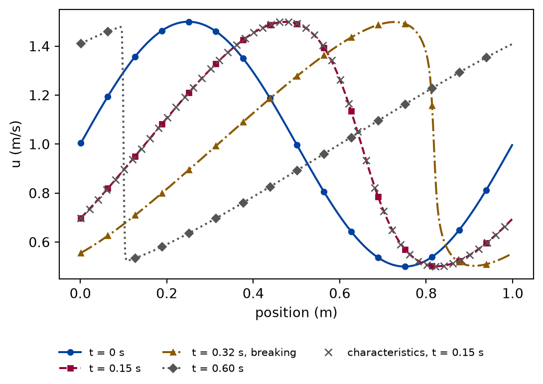
def draw_steepening() -> Figure:
    """The wave at four times, computed on four hundred cells: before the
    break with the characteristic solution beside it, at the break, and as a
    shock."""
    n = 400
    dx = LENGTH / n
    x = centres(n)
    t_break = the_breaking_time()
    times = [0.0, 0.15, t_break, 0.6]
    styles = [
        ("-", "o", FIGURE_COLOURS[0]),
        ("--", "s", FIGURE_COLOURS[1]),
        ("-.", "^", FIGURE_COLOURS[3]),
        (":", "D", FIGURE_COLOURS[2]),
    ]
    fig, ax = plt.subplots(figsize=(6.4, 4.4))
    u = initial(x)
    now = 0.0
    for t, (line, marker, colour) in zip(times, styles, strict=True):
        if t > now:
            u = evolve(u, dx, t - now, godunov(periodic), max_speed, COURANT).q
            now = t
        label = "t = 0 s" if t == 0 else f"t = {t:.2f} s"
        if t == t_break:
            label += ", breaking"
        ax.plot(
            x,
            u,
            color=colour,
            linestyle=line,
            marker=marker,
            markevery=25,
            markersize=4,
            label=label,
        )
    exact = characteristic_solution(initial, x[::8], 0.15, LENGTH)
    ax.plot(
        x[::8],
        exact,
        linestyle="none",
        marker="x",
        color=FIGURE_COLOURS[2],
        markersize=5,
        label="characteristics, t = 0.15 s",
    )
    ax.set_xlabel("position (m)")
    ax.set_ylabel("u (m/s)")
    fig.subplots_adjust(bottom=0.24)
    fig.legend(loc="lower center", ncol=3, frameon=False, fontsize=8)
    return fig

src/pbc/fluids/experiments/shock_waves_and_burgers_equation.py, lines 205 to 254, read from the repository when this page was built.

Figure 1: simulated A smooth wave of the Burgers equation steepens where it descends, becomes vertical at the breaking time, and then travels on as a shock; before the break the computed wave lies on the characteristic solution.

The crests travel faster than the troughs, so the front of each crest catches up with the trough ahead of it. At the breaking time the profile is vertical, and from then on it is a shock with a straight ramp behind it: the sawtooth that every periodic wave of this equation ends as. The run is simulated on four hundred cells; before the break the reference is the characteristic solution.

The speed of a shock

Four jumps, each from a left state $u_L$ to a right state $u_R$ with $u_L > u_R$ , start in the middle of a domain of one metre with open ends. The position of each shock, where the computed profile crosses the mean of the two states, is measured at two times, and the speed is their difference over the time between them.

pairs = [(2.0, 0.0), (1.0, -0.5), (3.0, 1.0), (1.0, -3.0)]  # u_L, u_R in m/s
SHOCK_CELLS = 400
DAM = 0.5  # m: where the jump starts
TRAVELS = (0.1, 0.3)  # m: the fastest wave travels this far by each of two times

src/pbc/fluids/experiments/shock_waves_and_burgers_equation.py, lines 43 to 46, read from the repository when this page was built.

def measured_speed(left: float, right: float, n: int = SHOCK_CELLS) -> float:
    """The speed of the shock between ``left`` and ``right``, from its
    positions at two times of the run."""
    dx = LENGTH / n
    x = centres(n)
    u = np.where(x < DAM, left, right)
    fastest = max(abs(left), abs(right))
    times = [d / fastest for d in TRAVELS]
    first = evolve(u, dx, times[0], godunov(transmissive), max_speed, COURANT).q
    second = evolve(
        first, dx, times[1] - times[0], godunov(transmissive), max_speed, COURANT
    ).q
    positions = [shock_position(v, x, left, right) for v in (first, second)]
    return (positions[1] - positions[0]) / (times[1] - times[0])

src/pbc/fluids/experiments/shock_waves_and_burgers_equation.py, lines 119 to 132, read from the repository when this page was built.

The speed of each shock measured from its positions at two times of a run on four hundred cells, against the jump of the flux over the jump of u.
left state (m/s)	right state (m/s)	measured speed (m/s)	Rankine-Hugoniot speed (m/s)
2.0	0.0	1.0000	1.0000
1.0	-0.5	0.2500	0.2500
3.0	1.0	1.9994	2.0000
1.0	-3.0	-1.0027	-1.0000

Numerically verified (Godunov scheme, four hundred cells, the four jumps of the table): A computed Burgers shock moves at the Rankine-Hugoniot speed, the mean of the two states. The largest difference is 0.09 per cent of the largest speed in the jump, with no knowledge of the shock speed in the scheme: the speed comes out of the fluxes, because the scheme conserves $u$ exactly. The shock in the last row moves to the left though the fluid on its left moves to the right: a shock is a wave, not a parcel of fluid.

The energy a shock destroys

The energy budget of the run, with what enters and leaves through the ends accounted for, gives the energy the scheme removed per unit time. For the smooth wave before it breaks, the exact solution removes none; for the shock from two metres per second to zero, it removes $(u_L - u_R)^3/12 =$ 0.6667 $\mathrm{m^3/s^3}$ .

ENERGY_PAIR = (2.0, 0.0)  # m/s
ENERGY_START = 0.2  # m
ENERGY_WINDOW = (0.05, 0.25)  # s
energy_cells = [100, 200, 400, 800]

src/pbc/fluids/experiments/shock_waves_and_burgers_equation.py, lines 50 to 53, read from the repository when this page was built.

def shock_energy_rate(n: int) -> float:
    """The rate at which the run removes energy while the shock of
    ``ENERGY_PAIR`` moves, from the energy budget over ``ENERGY_WINDOW``:
    what entered through the ends (u^3 / 3 at each) minus the growth of the
    energy in the domain."""
    left, right = ENERGY_PAIR
    dx = LENGTH / n
    x = centres(n)
    u = np.where(x < ENERGY_START, left, right)
    start, end = ENERGY_WINDOW
    first = evolve(u, dx, start, godunov(transmissive), max_speed, COURANT).q
    second = evolve(first, dx, end - start, godunov(transmissive), max_speed, COURANT).q
    entered = (left**3 - right**3) / 3.0
    return entered - (energy(second, dx) - energy(first, dx)) / (end - start)

src/pbc/fluids/experiments/shock_waves_and_burgers_equation.py, lines 161 to 174, read from the repository when this page was built.

The energy removed per unit time by the Godunov scheme, for each grid: from the smooth wave before it breaks, and from the shock between two and zero metres per second, where the energy that entered through the ends is accounted for.
cells	smooth wave (m³/s³)	shock (m³/s³)
100	0.00998	0.6688
200	0.00502	0.6662
400	0.00252	0.6664
800	0.00126	0.6669

Numerically verified (the shock and the smooth wave of the examples, Godunov scheme): The Godunov scheme removes energy at a shock at the rate $(u_L - u_R)^3/12$ whatever the grid, and from smooth flow at a rate that falls in proportion to the cell width. On the finest grid the shock rate differs from the closed form by 0.0 per cent. The two columns show two kinds of dissipation. In smooth flow it is the numerical diffusion of the previous lesson, an error of the grid that a finer grid removes. At a shock it is physics: the grid only decides over how many cells the energy is destroyed, not how much.

Limits

First order. The Godunov scheme of this lesson takes one value per cell on each side of a face. Schemes of higher order reconstruct a slope in each cell and need limiters near a shock; they are not built here.
Inviscid shocks. A real shock has a thickness set by viscosity and a structure inside it, which the inviscid limit replaces by a jump. The energy it destroys does not depend on that structure.
A scalar equation. Burgers’ equation has one wave. A system such as gas dynamics or shallow water has several, and its Riemann problem has several waves at once; the method carries over, the closed forms change.
Measured shock positions. The position is where the profile crosses the mean of the two states, interpolated between cells. A smeared shock makes that a measurement accurate to a fraction of a cell, which is why the speed is taken from two positions far apart.

Self-check. A smooth wave of the Burgers equation is computed on a very fine grid until long after it breaks. Does the total energy $\int u^2/2\,\mathrm{d}x$ of the computed solution stay constant as the grid is refined further?

Yes: the numerical dissipation vanishes as the cell width goes to zero, so on a fine enough grid the energy is conserved.

That holds before the break, where all the dissipation is numerical. After it the shock destroys energy at a rate set by the jump, not by the grid.
No: after the break the shock removes energy at the rate $(u_L - u_R)^3/12$ , which does not vanish as the grid is refined.

Correct: the dissipation at a shock is a property of the solution, the inviscid limit of a viscous fluid, and the grid only spreads it over a few cells.
No: the energy grows, because the shock steepens the profile.

A shock never adds energy; an entropy shock has $u_L > u_R$ , and the rate $(u_L - u_R)^3/12$ is then positive, a loss.

Solution to the self-check

No. Before the break the energy is conserved by the equation and lost only to the numerical diffusion, which a finer grid removes. After it the shock removes energy at the rate $(u_L - u_R)^3/12$ , which the solution itself fixes. The finest grid gives the same loss as a coarse one: the third example measured it at every resolution.

Exercises

Exercise 1. A fan instead of a shock. Start the Burgers equation from $u_L = 0$ on the left of $x_0 = 0.3$ m and $u_R = 1$ m/s on the right. The faster fluid is ahead, so no shock forms; the exact solution is the fan $u = (x - x_0)/t$ between the two states. Compute it on several grids and measure the order of the error.

Hint 1 of 1 for exercise 1

The fan has a corner at each end, where the slope jumps.

Solution to exercise 1

def rarefaction_run(experiment: Experiment) -> float:
    """Exercise 1: the rarefaction from u_L = 0 to u_R = 1 against the exact
    fan u = (x - x0) / t, for each grid; record the table, return the order."""
    start, t = 0.3, 0.4
    sizes = [100, 200, 400, 800]
    errors = []
    for n in sizes:
        dx = LENGTH / n
        x = centres(n)
        u = np.where(x < start, 0.0, 1.0)
        end = evolve(u, dx, t, godunov(transmissive), max_speed, COURANT).q
        exact = riemann_solution(0.0, 1.0, (x - start) / t)
        errors.append(float(np.sum(np.abs(end - exact)) * dx))
    experiment.table(
        "rarefaction-run",
        list(zip(sizes, errors, strict=True)),
        [("cells", "", "d"), ("error", "m²/s", ".3e")],
        "The error of the Godunov scheme against the exact rarefaction fan, "
        "the integral of the absolute difference over the domain, for each "
        "grid.",
    )
    return fitted_order(LENGTH / np.array(sizes), errors)

src/pbc/fluids/experiments/shock_waves_and_burgers_equation.py, lines 257 to 278, read from the repository when this page was built.

The error of the Godunov scheme against the exact rarefaction fan, the integral of the absolute difference over the domain, for each grid.
cells	error (m²/s)
100	9.389e-03
200	5.591e-03
400	3.258e-03
800	1.865e-03

The fitted order is 0.78, below the one of the smooth wave. The fan itself is a straight line, which the scheme follows well; the error comes from its two corners, where the profile has a kink that the numerical diffusion rounds. A first-order scheme converges more slowly at a kink than in smooth flow, and more slowly still at a jump that is not a shock.

Exercise 2. A shock that stands still. Start from $u_L = 1$ m/s and $u_R = -1$ m/s at $x_0 = 0.5$ m. Where is the shock after $0.3$ s?

Hint 1 of 1 for exercise 2

The Rankine-Hugoniot speed is the mean of the two states.

Solution to exercise 2

def standing_shock() -> tuple[float, float]:
    """Exercise 2: the shock between u_L = 1 and u_R = -1, its measured speed
    and its position after a while."""
    n = SHOCK_CELLS
    dx = LENGTH / n
    x = centres(n)
    u = np.where(x < DAM, 1.0, -1.0)
    end = evolve(u, dx, 0.3, godunov(transmissive), max_speed, COURANT).q
    return measured_speed(1.0, -1.0), shock_position(end, x, 1.0, -1.0)

src/pbc/fluids/experiments/shock_waves_and_burgers_equation.py, lines 281 to 289, read from the repository when this page was built.

The mean of the two states is zero, so the shock stands still. The run measures a speed of 0.0e+00 m/s, and the shock is at 0.5000 m after the run, where it started. The flux $u^2/2$ is the same on both sides of the jump, so conservation needs no motion of it. The characteristics run into the shock from both sides, and the energy they bring is destroyed there, at the rate of the third example.

Run this experiment

This page was built from commit 3a83ab640162bf2b624c2b254d917ed5bdc7090d of the repository.

In a clone at that commit, with the project’s Python packages installed, this command runs the experiment of this page:

uv run --locked --no-dev python -m pbc.fluids.experiments.shock_waves_and_burgers_equation results

Files, tests, and every command

The files behind it:

site/lessons/fluids/02-shock-waves-and-burgers-equation/index.qmd: this page, with every code cell.
src/pbc/fluids/burgers.py: code the experiment runs.
src/pbc/fluids/finite_volume.py: code the experiment runs.
src/pbc/fluids/experiments/shock_waves_and_burgers_equation.py: code the experiment runs.
src/pbc/verification/estimates.py: code the experiment runs.
src/pbc/experiment.py: code the experiment runs.
tests/unit/test_fluids.py: tests of that code.
tests/unit/test_shock_waves_and_burgers_equation_experiment.py: tests of that code.

With Git and uv installed (see the setup page), run:

git clone https://github.com/taspinar/physics-by-construction.git
cd physics-by-construction
git checkout 3a83ab640162bf2b624c2b254d917ed5bdc7090d
uv sync --locked --no-dev
uv run --locked --no-dev python -m pbc.fluids.experiments.shock_waves_and_burgers_equation results

The experiment writes every figure of this page into results/, as <label>.png, and every number and table of the page, as the page shows it, into results/results.json. Its numbers match this page to the digits shown, and its figure files are the ones the page shows; digits beyond those can differ between machines, because floating-point libraries differ. Change the code of the experiment and run it again to see what changes.