Advection and diffusion: schemes, stability, and the diffusion a grid adds

A quantity carried by a steady flow, computed with three difference schemes; the diffusion the upwind scheme adds measured from its runs and checked against its modified equation, the stability of each scheme against its Courant number, and a front fed through an inflow boundary.

Course

Fluid dynamics, lesson 1 of 4

Slot

FL1, Advection and diffusion

Methods

Simulation

Difficulty

Intermediate, level 2 of 3

What you’ll learn

Write the upwind, central, and Lax-Wendroff schemes for a quantity carried by a flow, with boundaries for an inflow and an outflow
Measure the diffusion a scheme adds and check it against the modified equation
Predict from the Courant and diffusion numbers whether a scheme is stable, and check it on the factor of each Fourier mode
Tell the physical diffusion of a model from the numerical diffusion of its grid

Prerequisites

Numerical integrators, Random walks and diffusion.

Before you begin

Calculus: partial derivatives, and Taylor expansion of a function of two variables
Complex numbers: the exponential of an imaginary number, and the modulus of a complex number

Related

none

Previous

Induction: magnetic flux and the electromotive force

Next

Shock waves and the Burgers equation

With scripts, this page keeps a record in your browser of whether you completed the lesson. Nothing is stored without them.

With scripts, this place suggests what to do next, with the reason, from the progress saved in your browser. Without them, follow the learning path.

A river carries a patch of dye downstream. The patch moves with the water, and it also spreads: molecules wander across the edges of the patch, and the sharp edges blur. The first is advection, transport by a flow; the second is diffusion. Smoke from a chimney, salt in an estuary, heat in a pipe, and a pollutant in the air all do both, and a model of any of them begins with the same equation.

The equation is linear and has an exact solution, so it is the place to learn what a grid does to it. A computer stores the dye only at points a cell width apart and advances it in steps. This lesson writes three schemes that do so, and asks three questions of them. How much does a scheme spread the dye on its own, with no diffusion in the physics? When does a scheme blow up? And what does a scheme need to know at the ends of the domain, where the water enters and leaves? Each answer is measured from the runs of the program and compared with a prediction made before the run.

Assumptions

One dimension, a steady and uniform flow. The water moves at one constant speed $a > 0$ everywhere. A real river is faster in the middle than at the banks, and that shear spreads a patch far more than molecular diffusion does; it is not in this lesson.
A passive quantity. The dye does not change the flow. Heat that makes the water rise, or a sediment heavy enough to slow it, would couple back.
Constant diffusion. The diffusion coefficient $\nu$ is the same everywhere. Turbulent mixing, which depends on the flow, is not.
A uniform grid and explicit steps. The cells are equal and each step uses only the values of the step before. An implicit scheme, which solves a system of equations each step, has other stability limits.
Smooth profiles for the modified equation. The prediction of the numerical diffusion is an expansion in the cell width; it describes a profile that varies over many cells, not the sharp edge of a square pulse.

The equation and three schemes

Advection and diffusion

A quantity $u(x, t)$ carried by a flow of speed $a$ and diffusing with the coefficient $\nu$ obeys

$\frac{\partial u}{\partial t} + a\,\frac{\partial u}{\partial x} = \nu\,\frac{\partial^2 u}{\partial x^2}.$

Without diffusion the solution is the initial profile moved downstream, $u(x, t) = u_0(x - a t)$ : nothing spreads. With diffusion alone a sine of wavenumber $k$ keeps its shape and decays as $\mathrm{e}^{-\nu k^2 t}$ ; short waves die fast, which is why sharp edges blur first. With both, the sine moves at the speed $a$ and decays at the rate $\nu k^2$ .

A grid and a step

The program keeps $u_j^n$ , the value in cell $j$ after $n$ steps, on cells of width $\Delta x$ with steps $\Delta t$ . Two numbers decide how a scheme behaves:

$C = \frac{a\,\Delta t}{\Delta x}, \qquad r = \frac{\nu\,\Delta t}{\Delta x^2}.$

The Courant number $C$ is the fraction of a cell the flow crosses in one step; the diffusion number $r$ plays the same part for diffusion. Each scheme below updates a cell from itself and its two neighbours:

$\begin{aligned} \text{upwind:}\quad & u_j^{n+1} = u_j^n - C\,(u_j^n - u_{j-1}^n), \\ \text{central:}\quad & u_j^{n+1} = u_j^n - \tfrac{C}{2}\,(u_{j+1}^n - u_{j-1}^n), \\ \text{Lax-Wendroff:}\quad & u_j^{n+1} = u_j^n - \tfrac{C}{2}\,(u_{j+1}^n - u_{j-1}^n) + \tfrac{C^2}{2}\,(u_{j+1}^n - 2u_j^n + u_{j-1}^n), \end{aligned}$

and the diffusion adds $r\,(u_{j+1}^n - 2u_j^n + u_{j-1}^n)$ . The upwind scheme takes the difference on the side the flow comes from; the central scheme on both sides; Lax-Wendroff adds the term that makes it exact to second order in $\Delta t$ for a smooth profile.

The modified equation

What equation does the upwind scheme actually solve? Expand each value in a Taylor series about $(x_j, t_n)$ , $u_{j-1} = u - \Delta x\,u_x + \tfrac12 \Delta x^2 u_{xx} - \dots$ and $u^{n+1} = u + \Delta t\,u_t + \tfrac12 \Delta t^2 u_{tt} + \dots$ , and put them into the scheme. Using $u_{tt} = a^2 u_{xx}$ from the equation itself, the scheme agrees to second order with

$\frac{\partial u}{\partial t} + a\,\frac{\partial u}{\partial x} = \left(\nu + \frac{a\,\Delta x}{2}\,(1 - C)\right)\frac{\partial^2 u}{\partial x^2}.$

The upwind scheme diffuses with the extra coefficient $\nu_{\text{num}} = a\,\Delta x\,(1 - C)/2$ , whether the physics has any diffusion or not. It is proportional to the cell width, so it falls as the grid is refined, and it vanishes at $C = 1$ , where each step moves the profile by exactly one cell. The next term of the expansion is of order $\Delta x^2$ , so a measured diffusion should differ from $\nu_{\text{num}}$ by a relative amount that falls as $\Delta x^2$ . That is the first prediction the lesson tests.

Stability

Put a single Fourier mode $u_j^n = G^n \mathrm{e}^{\mathrm{i} j \theta}$ into a scheme: every scheme above returns the same mode times a factor $G(\theta)$ , the amplification factor. A scheme is stable when $|G| \le 1$ for every $\theta$ ; otherwise the mode with the largest $|G|$ grows each step until it swamps the solution (von Neumann’s condition). For the three schemes, each with the diffusion added,

$\begin{aligned} \text{upwind:}\quad & G = 1 - C\,(1 - \mathrm{e}^{-\mathrm{i}\theta}) - 2r\,(1 - \cos\theta), \\ \text{central:}\quad & G = 1 - 2r\,(1 - \cos\theta) - \mathrm{i}\,C \sin\theta, \\ \text{Lax-Wendroff:}\quad & G = 1 - (C^2 + 2r)(1 - \cos\theta) - \mathrm{i}\,C \sin\theta . \end{aligned}$

With $x = 1 - \cos\theta$ , which runs from $0$ to $2$ , and $\sin^2\theta = x\,(2 - x)$ , the last two give

$\begin{aligned} \text{central:}\quad & |G|^2 = 1 - 2x\,(2r - C^2) + x^2\,(4r^2 - C^2), \\ \text{Lax-Wendroff:}\quad & |G|^2 = 1 - 4r\,x + x^2\left((C^2 + 2r)^2 - C^2\right). \end{aligned}$

Each is $1$ plus $x$ times a function linear in $x$ , so $|G| \le 1$ for every mode exactly when that function is not positive at both ends, at the long waves, $x \to 0$ , and at the sawtooth, $\theta = \pi$ , $x = 2$ . The upwind scheme is stable for $C + 2r \le 1$ : the worst mode is the sawtooth, with $G = 1 - 2(C + 2r)$ . Lax-Wendroff is stable for $C^2 + 2r \le 1$ , with the sawtooth again the worst mode, $G = 1 - 2(C^2 + 2r)$ ; without diffusion that is $C \le 1$ . The central scheme is stable for $C^2 \le 2r \le 1$ : the long waves grow unless $C^2 \le 2r$ , the sawtooth unless $r \le 1/2$ . Without diffusion it grows for every $C > 0$ ; enough diffusion damps that growth, though not more than $r = 1/2$ , where the diffusion breaks the scheme on its own. With $r = 0$ the limit of upwind and Lax-Wendroff is $C \le 1$ , the Courant-Friedrichs-Lewy condition: in one step the flow must not carry the quantity further than the scheme looks, one cell. Diffusion only narrows it.

Boundaries

At the ends of a finite domain a scheme needs the value beyond the last cell, which the program supplies as a ghost cell. Where the flow enters, the ghost holds what the flow brings in: an inflow value is physics. Where it leaves, the flow takes the quantity away and nothing comes back, so the exact solution needs no condition at all. The upwind scheme agrees: it never reads the cell downstream. Lax-Wendroff and the central scheme read both neighbours, so they need a value at the outflow that the physics does not give, and a wrong one sends an error back into the domain.

Code

step applies a scheme to every cell at once, with the ghost cells of the boundary; amplification measures the factor of each Fourier mode by applying one step to the mode itself, and modified_diffusion is the coefficient of the modified equation.

def step(
    u: Array,
    courant: float,
    scheme: str,
    boundary: Boundary = periodic,
    diffusion: float = 0.0,
) -> Array:
    """One step of ``scheme`` (a key of ``SCHEMES``) at the Courant number
    ``courant``, plus the explicit central diffusion r (u_left - 2 u +
    u_right) for the diffusion number ``diffusion``."""
    padded = with_ghosts(u, boundary)
    left, right = padded[:-2], padded[2:]
    advected = SCHEMES[scheme](left, u, right, courant)
    return advected + diffusion * (left - 2.0 * u + right)

src/pbc/fluids/advection.py, lines 61 to 74, read from the repository when this page was built.

def amplification(
    scheme: str, courant: float, n: int, diffusion: float = 0.0
) -> NDArray[np.complex128]:
    """The factor by which one step multiplies each Fourier mode of a periodic
    grid of ``n`` cells, measured by applying the step to the mode
    exp(i j theta) itself, theta = 2 pi k / n for k = 0 .. n - 1. A scheme is
    stable when no factor exceeds one in modulus."""
    j = np.arange(n)
    factors = np.empty(n, dtype=complex)
    for k in range(n):
        mode = np.exp(2j * np.pi * k * j / n)
        factors[k] = step(mode, courant, scheme, periodic, diffusion)[0] / mode[0]
    return factors

src/pbc/fluids/advection.py, lines 97 to 109, read from the repository when this page was built.

def modified_diffusion(speed: float, dx: float, courant: float) -> float:
    """The numerical diffusion a dx (1 - C) / 2 of the upwind scheme (m^2/s
    for a in m/s and dx in m): the coefficient of u_xx in its modified
    equation, which the scheme adds to the physical diffusion."""
    return speed * dx * (1.0 - courant) / 2.0

src/pbc/fluids/advection.py, lines 120 to 124, read from the repository when this page was built.

Worked examples

The diffusion of the upwind scheme

A sine of one wave is carried once across a periodic domain by the upwind scheme, with no physical diffusion, on grids of twenty-five to four hundred cells. Its amplitude after the run gives the diffusion the scheme added, $D = -\ln(A_{\text{end}}/A_{\text{start}})/(k^2 T)$ , which is compared with $\nu_{\text{num}}$ of the modified equation.

SPEED = 1.0  # m/s
LENGTH = 1.0  # m, a periodic domain
COURANT = 0.5
cells = [25, 50, 100, 200, 400]
WAVE = 1  # whole waves of the sine over the domain
DURATION = 1.0  # s: the wave crosses the domain once

src/pbc/fluids/experiments/advection_and_diffusion.py, lines 33 to 38, read from the repository when this page was built.

def measured_diffusion(
    n: int, viscosity: float = 0.0, courant: float = COURANT
) -> float:
    """Advect a sine of one wave across the periodic domain once with the
    upwind scheme on ``n`` cells at the Courant number ``courant``, and
    return the diffusion coefficient that its loss of amplitude implies,
    A(T) = A(0) exp(-D k^2 T)."""
    dx = LENGTH / n
    dt = courant * dx / SPEED
    k = 2.0 * np.pi * WAVE / LENGTH
    start = np.sin(k * centres(n))
    end = advect(
        start,
        courant,
        "upwind",
        round(DURATION / dt),
        diffusion=viscosity * dt / dx**2,
    )
    ratio = mode_amplitude(end, WAVE) / mode_amplitude(start, WAVE)
    return -np.log(ratio) / (k * k * DURATION)

src/pbc/fluids/experiments/advection_and_diffusion.py, lines 91 to 110, read from the repository when this page was built.

The diffusion coefficient implied by the loss of amplitude of a sine advected once across the domain by the upwind scheme at a Courant number of one half, against the coefficient of its modified equation, for each grid.
cells	cell width (m)	measured diffusion (m²/s)	modified equation (m²/s)	relative difference
25	0.0400	1.0026e-02	1.0000e-02	2.64e-03
50	0.0200	5.0033e-03	5.0000e-03	6.59e-04
100	0.0100	2.5004e-03	2.5000e-03	1.65e-04
200	0.0050	1.2501e-03	1.2500e-03	4.11e-05
400	0.0025	6.2501e-04	6.2500e-04	1.03e-05

Numerically verified (upwind scheme, a sine of one wave, Courant number one half, periodic domain): The upwind scheme diffuses a smooth profile with the coefficient $a\,\Delta x\,(1 - C)/2$ of its modified equation; the measured and predicted coefficients differ by a relative amount that falls as the square of the cell width. The fitted order of the relative difference is 2.001. The measured diffusion halves with the cell width, as a first-order scheme must: on the coarsest grid the sine loses 33 per cent of its amplitude in one crossing, though the equation that was meant to be solved keeps it forever. The data are simulated, and the reference is the modified equation, derived before the run.

Physical diffusion under numerical diffusion

The same sine on one hundred cells, now with a physical diffusion added to the upwind scheme, for viscosities from two thousandths of a square metre per second down to zero.

PHYSICAL_CELLS = 100
viscosities = [2e-3, 1e-3, 3e-4, 1e-4, 0.0]  # m^2/s

src/pbc/fluids/experiments/advection_and_diffusion.py, lines 42 to 43, read from the repository when this page was built.

The diffusion measured from the upwind scheme with an explicit physical diffusion on one hundred cells, against the viscosity plus the numerical diffusion of the modified equation, and the ratio of the numerical to the physical part.
viscosity (m²/s)	viscosity plus numerical (m²/s)	measured diffusion (m²/s)	numerical over physical
2.0e-03	4.5000e-03	4.5001e-03	1.25
1.0e-03	3.5000e-03	3.5002e-03	2.50
3.0e-04	2.8000e-03	2.8003e-03	8.33
1.0e-04	2.6000e-03	2.6004e-03	25.00
0.0e+00	2.5000e-03	2.5004e-03

Numerically verified (upwind scheme with explicit central diffusion, one hundred cells, Courant number one half): With a physical diffusion $\nu$ , the upwind scheme diffuses with $\nu + a\,\Delta x\,(1 - C)/2$ : the two add. At the smallest viscosity the grid adds 25 times more diffusion than the physics. A run on this grid of a flow with that viscosity computes the diffusion of the grid and calls it the flow. Before a simulation of a slightly diffusive flow is believed, the numerical diffusion has to be estimated and shown to be smaller than the physical one, as the first exercise does.

Stability and the Courant number

Each scheme is run for two hundred steps from a square pulse of height one, at the Courant and diffusion numbers of the table, and the factor of every Fourier mode of the grid is measured by applying one step to it.

STABILITY_CELLS = 64
STABILITY_STEPS = 200
runs = [
    ("upwind", 0.5, 0.0),
    ("upwind", 1.0, 0.0),
    ("upwind", 1.1, 0.0),
    ("Lax-Wendroff", 0.9, 0.0),
    ("Lax-Wendroff", 1.1, 0.0),
    ("central", 0.5, 0.0),
    ("upwind", 0.5, 0.25),
    ("upwind", 0.5, 0.3),
    ("central", 0.5, 0.25),
    ("central", 0.8, 0.1),
    ("central", 0.5, 0.6),
    ("Lax-Wendroff", 0.5, 0.3),
    ("Lax-Wendroff", 0.9, 0.2),
]  # scheme, Courant number C, diffusion number r

src/pbc/fluids/experiments/advection_and_diffusion.py, lines 47 to 63, read from the repository when this page was built.

For each scheme, Courant number and diffusion number: the largest modulus of the factor by which one step multiplies a Fourier mode of a grid of sixty-four cells, measured by applying the step to each mode, and the largest value of a square pulse of height one after two hundred steps.
scheme	Courant number	diffusion number	largest factor per step	largest value after the steps
upwind	0.5	0.00	1.0000	0.711
upwind	1.0	0.00	1.0000	1.000
upwind	1.1	0.00	1.2000	3.5e+14
Lax-Wendroff	0.9	0.00	1.0000	1.166
Lax-Wendroff	1.1	0.00	1.4200	9.5e+28
central	0.5	0.00	1.1180	4.7e+08
upwind	0.5	0.25	1.0000	0.486
upwind	0.5	0.30	1.2000	1.9e+14
central	0.5	0.25	1.0000	0.711
central	0.8	0.10	1.1499	8.0e+10
central	0.5	0.60	1.4000	4.6e+27
Lax-Wendroff	0.5	0.30	1.0000	0.506
Lax-Wendroff	0.9	0.20	1.4200	8.8e+28

Numerically verified (the three schemes on a periodic grid of sixty-four cells, the Courant and diffusion numbers of the table): The upwind scheme is stable for $C + 2r \le 1$ , Lax-Wendroff for $C^2 + 2r \le 1$ , and the central scheme for $C^2 \le 2r \le 1$ , so for no $C > 0$ without diffusion; where the largest factor exceeds one, the pulse grows without bound. The factors measured by the program are the closed forms of the explanation: $2(C + 2r) - 1$ for upwind and $2(C^2 + 2r) - 1$ for Lax-Wendroff beyond their limits, at the sawtooth; for the central scheme $\sqrt{1 + C^2}$ without diffusion, at $\theta = \pi/2$ , $4r - 1$ at the sawtooth for $r = 0.6$ , and the largest $|G|$ of the closed form over the modes of the grid for $C = 0.8$ , $r = 0.1$ , where the growing modes are the long waves. A diffusion number that is too large breaks the upwind scheme even at a safe Courant number, and Lax-Wendroff at $C = 0.9$ , stable on its own, breaks with $r = 0.2$ . The central scheme, unstable on its own, is stable at $C = 0.5$ with $r = 0.25$ and not at $C = 0.8$ with $r = 0.1$ , though $C$ is below one there: diffusion damps its growth only where $C^2 \le 2r$ . Lax-Wendroff is stable at $C$ below one yet its largest value exceeds the height of the pulse: stability bounds the growth of the modes, not the overshoot at an edge, which the figure below shows.

A front fed through the inflow

The domain now has ends. The left end is an inflow that brings $u = 1$ ; the right end is an open outflow. At the start the domain holds a front, $u = 1$ behind it and $u = 0$ ahead, and the upwind scheme carries it downstream. The exact solution is the sharp front moved by $a\,t$ . The modified equation predicts a smeared front instead, the error function of a front that diffuses with $\nu_{\text{num}}$ :

$u(x, t) = \tfrac12\,\operatorname{erfc}\!\left(\frac{x - x_0 - a\,t}{2\sqrt{\nu_{\text{num}}\,t}}\right).$

front_cells = [40, 80, 160, 320, 640]
FRONT_START = 0.25  # m: the front at the start; behind it u = 1, ahead u = 0
FRONT_TIME = 0.5  # s

src/pbc/fluids/experiments/advection_and_diffusion.py, lines 67 to 69, read from the repository when this page was built.

def front_profile(n: int) -> tuple[np.ndarray, np.ndarray, np.ndarray]:
    """The upwind run of a front that the inflow keeps fed, on ``n`` cells:
    the centres, the computed profile, and the error-function front of the
    modified equation."""
    dx = LENGTH / n
    x = centres(n)
    start = np.where(x < FRONT_START, 1.0, 0.0)
    end = advect(
        start,
        COURANT,
        "upwind",
        round(FRONT_TIME / (COURANT * dx / SPEED)),
        boundary=inflow_outflow(1.0),
    )
    d = modified_diffusion(SPEED, dx, COURANT)
    smeared = 0.5 * erfc(
        (x - FRONT_START - SPEED * FRONT_TIME) / (2.0 * np.sqrt(d * FRONT_TIME))
    )
    return x, end, smeared

src/pbc/fluids/experiments/advection_and_diffusion.py, lines 221 to 239, read from the repository when this page was built.

The largest difference between the upwind profile of a front fed by the inflow boundary and two references, for each grid: the sharp front of the exact advection, and the error-function front of the modified equation.
cells	largest difference from the sharp front	largest difference from the modified equation
40	0.437	6.78e-04
80	0.456	3.41e-04
160	0.469	1.70e-04
320	0.478	8.49e-05
640	0.484	4.25e-05

Numerically verified (upwind scheme, Courant number one half, an inflow value of one, the start and duration of the example): The upwind front fed by the inflow differs from the sharp front by nearly half its height at every resolution, and from the error-function front of the modified equation by an amount that falls in proportion to the cell width. The fitted order of the second difference is 1.00. The front never gets sharper than the grid allows: the width of the smeared front, $\sqrt{\nu_{\text{num}} t}$ , falls only as the square root of the cell width, so the largest difference from the sharp front shrinks very slowly, and at the front itself never. The inflow boundary keeps the domain fed: the region behind the front stays at the inflow value.

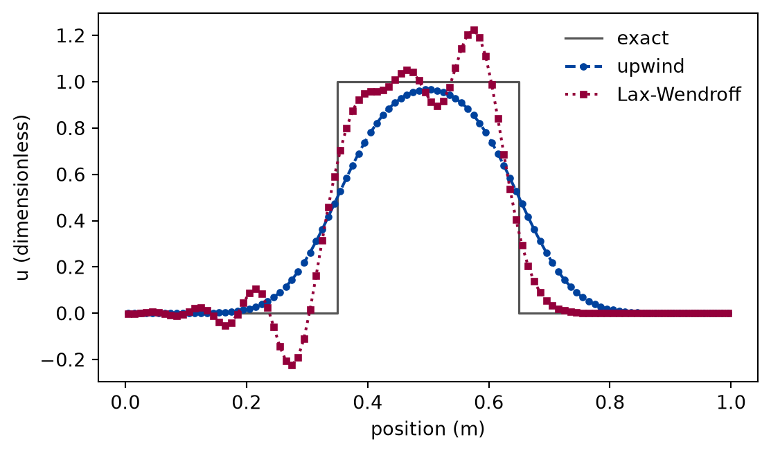
def draw_advected_pulse() -> Figure:
    """A square pulse carried once around the periodic domain by the upwind
    and the Lax-Wendroff schemes, against the exact profile, which is the
    pulse where it started."""
    n = 100
    x = centres(n)
    pulse = np.where(np.abs(x - 0.5) < 0.15, 1.0, 0.0)
    steps = round(DURATION / (COURANT * LENGTH / n / SPEED))
    upwind = advect(pulse, COURANT, "upwind", steps)
    lax_wendroff = advect(pulse, COURANT, "Lax-Wendroff", steps)
    fig, ax = plt.subplots(figsize=(6.4, 3.6))
    ax.plot(
        x,
        pulse,
        color=FIGURE_COLOURS[2],
        linewidth=1.2,
        drawstyle="steps-mid",
        label="exact",
    )
    ax.plot(
        x,
        upwind,
        color=FIGURE_COLOURS[0],
        linestyle="--",
        marker="o",
        markersize=3,
        label="upwind",
    )
    ax.plot(
        x,
        lax_wendroff,
        color=FIGURE_COLOURS[1],
        linestyle=":",
        marker="s",
        markersize=3,
        label="Lax-Wendroff",
    )
    ax.set_xlabel("position (m)")
    ax.set_ylabel("u (dimensionless)")
    ax.legend(loc="upper right", frameon=False)
    return fig

src/pbc/fluids/experiments/advection_and_diffusion.py, lines 275 to 315, read from the repository when this page was built.

Figure 1: simulated A square pulse carried once around a periodic domain: the upwind scheme smears its edges, Lax-Wendroff keeps them steeper but rings around them, and neither returns the pulse it started from.

The figure shows the two errors a scheme can make. The upwind scheme is monotone: it makes no new maximum or minimum, and pays for it with the diffusion of its modified equation. Lax-Wendroff has no numerical diffusion at second order, and its leading error is dispersion: waves of different lengths travel at different speeds, and the short waves of the edges fall behind and ring. The run is simulated on one hundred cells, and the reference is the exact solution, the pulse where it started.

Limits

A model equation. Real advection happens in a flow that changes in space and time, in three dimensions; the schemes carry over, the closed forms of this lesson do not.
The modified equation is an expansion. It predicts the diffusion of a profile resolved by many cells. A sharp edge has components at every wavelength, down to the cell width, where the expansion fails; the stability factors, not the modified equation, decide what happens there.
Von Neumann’s condition is for a periodic, uniform grid. Boundaries and variable coefficients can make a scheme unstable that passes it, which is why the stability examples run the schemes as well as compute the factors.
Only explicit schemes. An implicit scheme can take larger steps but still adds its own numerical diffusion; that trade is not measured here.

Self-check. On a fixed grid, with the upwind scheme and no physical diffusion, you halve the time step to make the run more accurate. What happens to the numerical diffusion?

It halves, because the error of an explicit scheme is proportional to the time step.

The local error of a step does shrink, but the numerical diffusion is $a\,\Delta x\,(1 - C)/2$ , and halving the step halves $C$ : the factor $1 - C$ grows.
It grows, because the Courant number falls and the factor $1 - C$ rises.

Correct: with the cell width fixed, the smaller step moves the scheme away from $C = 1$ , where the upwind scheme is exact, and the profile diffuses more.
It does not change, because it depends only on the cell width.

It depends on the cell width and on the Courant number; the time step enters through $C$ .

Solution to the self-check

It grows. The numerical diffusion of the upwind scheme is $a\,\Delta x\,(1 - C)/2$ , largest for small steps, at $\Delta x\,a/2$ , and zero at $C = 1$ . A smaller step makes more steps, each of which smears the profile over the same cell width. The way to less numerical diffusion is a finer grid or a scheme of higher order, not a smaller step.

Exercises

Exercise 1. A grid fine enough for the physics. A dye diffuses with $\nu = 10^{-2}\ \mathrm{m^2/s}$ in a flow of $1$ m/s, on a periodic domain of $1$ m. Choose a number of cells and a time step so that the numerical diffusion of the upwind scheme is at most a tenth of $\nu$ and the scheme is stable, and check the diffusion the run measures.

Hint 1 of 2 for exercise 1

Since $1 - C$ is at most one, a cell width with $a\,\Delta x/2 \le \nu/10$ is enough whatever the step.

Hint 2 of 2 for exercise 1

With diffusion the stability limit is $C + 2r \le 1$ ; solve it for the step.

Solution to exercise 1

def grid_for(viscosity: float) -> tuple[int, int, float, float, float, float]:
    """Exercise 1: a grid and a step on which the numerical diffusion of the
    upwind scheme is at most a tenth of ``viscosity`` and the scheme is
    stable. Return the cells, the steps over the duration, the Courant and
    diffusion numbers, the numerical diffusion, and the diffusion measured."""
    # a dx (1 - C) / 2 < a dx / 2 <= nu / 10 holds for every C when dx <= nu / (5 a)
    n = int(np.ceil(LENGTH * 5.0 * SPEED / viscosity))
    dx = LENGTH / n
    # the stability limit C + 2 r <= 1 is dt <= 1 / (a / dx + 2 nu / dx^2)
    steps = int(np.ceil(DURATION * (SPEED / dx + 2.0 * viscosity / dx**2)))
    courant = SPEED * DURATION / steps / dx
    r = viscosity * DURATION / steps / dx**2
    assert courant + 2.0 * r <= 1.0, "the step breaks the stability limit"
    numerical = modified_diffusion(SPEED, dx, courant)
    assert numerical <= viscosity / 10.0, "the numerical diffusion is too large"
    return n, steps, courant, r, numerical, measured_diffusion(n, viscosity, courant)

src/pbc/fluids/experiments/advection_and_diffusion.py, lines 318 to 333, read from the repository when this page was built.

A cell width of $\nu/(5a)$ gives 500 cells. The stability limit, $\Delta t \le 1/(a/\Delta x + 2\nu/\Delta x^2)$ , then needs 5500 steps to cross the domain once: a Courant number of 0.0909 and a diffusion number of 0.4545. Diffusion, not advection, sets the step. The numerical diffusion is 9.091e-04 $\mathrm{m^2/s}$ , and the run measures 1.0909e-02 $\mathrm{m^2/s}$ , the viscosity plus that. Taking the step of the advection alone, a Courant number of one half, would have broken the stability limit.

Exercise 2. The Courant number one. Run the upwind scheme at $C = 1$ with no diffusion. What does the modified equation predict, and what does the run show?

Solution to exercise 2

def courant_one() -> float:
    """Exercise 2: the diffusion measured with the upwind scheme at a Courant
    number of one, where each step moves the profile by exactly one cell."""
    n = PHYSICAL_CELLS
    k = 2.0 * np.pi * WAVE / LENGTH
    start = np.sin(k * centres(n))
    end = advect(start, 1.0, "upwind", round(DURATION * SPEED * n / LENGTH))
    return abs(mode_amplitude(end, WAVE) / mode_amplitude(start, WAVE) - 1.0)

src/pbc/fluids/experiments/advection_and_diffusion.py, lines 336 to 343, read from the repository when this page was built.

At $C = 1$ the scheme is $u_j^{n+1} = u_{j-1}^n$ : every step moves the profile by exactly one cell, which is the exact solution. The modified equation gives $\nu_{\text{num}} = 0$ , and the run changes the amplitude of the sine by less than 1e-12. The exactness is fragile: a flow whose speed varies from place to place has no single step with $C = 1$ in every cell.

Exercise 3. Which schemes need an outflow condition? Carry a narrow pulse out through the right end of a domain with the upwind and with the Lax-Wendroff scheme, once with an open outflow and once with the value zero fixed beyond it. Which scheme notices the difference?

Hint 1 of 1 for exercise 3

Look at which neighbours each scheme reads.

Solution to exercise 3

def outflow_run(experiment: Experiment) -> list[float]:
    """Exercise 3: a pulse carried out through the right end, once with the
    open outflow and once with a fixed value zero beyond it, for the upwind
    and the Lax-Wendroff schemes; record the largest difference of the two
    runs while the pulse leaves."""
    n = 200
    x = centres(n)
    pulse = np.exp(-(((x - 0.5) / 0.02) ** 2))
    steps = round(0.5 / (0.8 * LENGTH / n / SPEED))  # the pulse at the outflow
    differences = []
    for scheme in ("upwind", "Lax-Wendroff"):
        open_end = advect(pulse, 0.8, scheme, steps, boundary=inflow_outflow(0.0))
        closed = advect(pulse, 0.8, scheme, steps, boundary=fixed(0.0, 0.0))
        differences.append(float(np.max(np.abs(open_end - closed))))
    assert differences[0] == 0.0, "the upwind scheme read the outflow ghost"
    assert differences[1] > 1e-6, "Lax-Wendroff did not read the outflow ghost"
    experiment.table(
        "outflow-run",
        [("upwind", "exactly zero"), ("Lax-Wendroff", f"{differences[1]:.2e}")],
        [("scheme", "", ""), ("largest difference of the two runs", "", "")],
        "The largest difference between a run with an open outflow and a run "
        "with a fixed value zero beyond the outflow end, when a pulse reaches "
        "it, for each scheme.",
    )
    return differences

src/pbc/fluids/experiments/advection_and_diffusion.py, lines 346 to 370, read from the repository when this page was built.

The largest difference between a run with an open outflow and a run with a fixed value zero beyond the outflow end, when a pulse reaches it, for each scheme.
scheme	largest difference of the two runs
upwind	exactly zero
Lax-Wendroff	8.56e-02

The upwind runs are identical to the last bit: the scheme reads only the neighbour upstream, so the value beyond the outflow never enters the computation, as the exact solution says it should not. Lax-Wendroff reads it, and a fixed zero there changes the solution as the pulse reaches the end. A scheme that reads downstream needs an outflow condition that the physics does not supply, and an extrapolation such as copying the last cell is the usual choice.

Run this experiment

This page was built from commit 3a83ab640162bf2b624c2b254d917ed5bdc7090d of the repository.

In a clone at that commit, with the project’s Python packages installed, this command runs the experiment of this page:

uv run --locked --no-dev python -m pbc.fluids.experiments.advection_and_diffusion results

Files, tests, and every command

The files behind it:

site/lessons/fluids/01-advection-and-diffusion/index.qmd: this page, with every code cell.
src/pbc/fluids/advection.py: code the experiment runs.
src/pbc/fluids/finite_volume.py: code the experiment runs.
src/pbc/fluids/experiments/advection_and_diffusion.py: code the experiment runs.
src/pbc/verification/estimates.py: code the experiment runs.
src/pbc/experiment.py: code the experiment runs.
tests/unit/test_fluids.py: tests of that code.
tests/unit/test_advection_and_diffusion_experiment.py: tests of that code.

With Git and uv installed (see the setup page), run:

git clone https://github.com/taspinar/physics-by-construction.git
cd physics-by-construction
git checkout 3a83ab640162bf2b624c2b254d917ed5bdc7090d
uv sync --locked --no-dev
uv run --locked --no-dev python -m pbc.fluids.experiments.advection_and_diffusion results

The experiment writes every figure of this page into results/, as <label>.png, and every number and table of the page, as the page shows it, into results/results.json. Its numbers match this page to the digits shown, and its figure files are the ones the page shows; digits beyond those can differ between machines, because floating-point libraries differ. Change the code of the experiment and run it again to see what changes.