The collision rule of two hard spheres from the momentum lesson, stated in Lean 4, with a proof that it conserves the total momentum along every axis for every choice of masses, velocities, and direction.
With scripts, this page keeps a record in your browser of whether you completed the lesson. Nothing is stored without them.
With scripts, this place suggests what to do next, with the reason, from the progress saved in your browser. Without them, follow the learning path.
The momentum lesson ran collisions and found that the total momentum of the pair was the same before and after, to round-off. That is what a program reports for the collisions it ran. A collision rule is supposed to conserve momentum for every pair of masses, every pair of velocities, and every direction of contact, and a run cannot cover them all.
This lesson takes the rule that the momentum lesson uses for hard spheres, hard_sphere_collision, writes it down in Lean, and proves that it conserves the total momentum. The proof is a short piece of algebra, and the compiler checks it for all real numbers at once. The lesson says what the theorem is about, how it connects to the numbers the simulation printed, and what it leaves unproved.
Assumptions
The model is two particles that collide once, and the rule that gives their velocities afterwards. Each assumption is a hypothesis or a definition in the Lean text, not an axiom, and the build fails on sorry and on any axiom the project declares.
The rule is the one of the momentum lesson. The velocity of the first sphere changes by a multiple of the direction n, and the multiple is times the component of the relative velocity along n; the second sphere changes by times the same. These are the definitions firstAfter and secondAfter. A rule with other coefficients is another definition, and the theorem says nothing about it.
Positive masses.hm₁ : 0 < m₁ and hm₂ : 0 < m₂. They make the sum non-zero, which the rule divides by, and they say that the spheres are particles.
Any number of axes. The velocities are vectors with one real number per axis (ι → ℝ with a finite set of axes ι), so the theorem holds on a line, in a plane, and in space.
Any direction. The direction n is an arbitrary vector. The momentum is conserved whether or not n has length one; the unit length matters for the energy and for the physical meaning of n as the line of centres, and neither is part of this theorem.
Real numbers, not floating-point numbers. Lean’s ℝ has no round-off. The program computes with doubles, and the theorem describes the model that it approximates.
The collision is instantaneous. The rule gives the velocities before and after, and says nothing about the contact in between. The soft contact of the momentum lesson, a force that acts for a short time, is a different model and is not proved here.
What the theorem says
The total momentum of two particles is . The collision rule changes both velocities by multiples of the same direction :
The change of momentum of the first sphere is times a vector, and that of the second is times the same vector: equal and opposite. The sum of the two cannot change, and the proof checks it by clearing the denominator and cancelling.
Formal theorem (the instantaneous collision rule of two hard spheres, real arithmetic): For two particles of positive mass, the collision rule conserves the total momentum along every axis, for all velocities and every direction.
Formal theorem (the same rule, real arithmetic): The change of momentum of the first sphere is the negative of the change of momentum of the second.
The first statement is what the simulation of the momentum lesson observed. The second is the reason: a force between two bodies acts on both, and the rule is the net effect of that force.
The proofs
The listings are read from the Lean files of the repository when the site is built, and they are the text that lake build compiled. The box says which commit, which version of Lean, and which version of Mathlib did it.
Compiled with Lean 4.34.1 and Mathlib v4.34.1: ./scripts/check-lean.sh found no sorry and no axiom declared by the project before this page was built.
./scripts/check-lean.sh ran lake build on every module of the project and found no sorry and no axiom declared by the project before this page was built. CI runs the same check on every pull request and on main.
Lean 4.34.1, from the toolchain pinned in lean/lean-toolchain.
The file in the repository at that commit and the result of the CI run are authoritative. The Lean web editor is a convenience: it runs its own version of Mathlib, which can differ from the one above, so a proof that compiled here may report an error there.
The rule itself comes first. dot is the scalar product, a sum over the axes; firstAfter and secondAfter return the velocity along each axis i.
/-- The scalar product of two vectors of `ι → ℝ`. -/def dot {ι : Type*} [Fintype ι] (a b : ι → ℝ) : ℝ := ∑ i, a i * b i/-- The velocity of the first sphere after the collision:`v₁' = v₁ - 2 m₂ / (m₁ + m₂) ((v₁ - v₂) · n) n`. -/noncomputabledef firstAfter {ι : Type*} [Fintype ι] (m₁ m₂ : ℝ) (v₁ v₂ n : ι → ℝ) : ι → ℝ :=fun i => v₁ i - 2 * m₂ / (m₁ + m₂) * dot (fun j => v₁ j - v₂ j) n * n i/-- The velocity of the second sphere after the collision:`v₂' = v₂ + 2 m₁ / (m₁ + m₂) ((v₁ - v₂) · n) n`. -/noncomputabledef secondAfter {ι : Type*} [Fintype ι] (m₁ m₂ : ℝ) (v₁ v₂ n : ι → ℝ) : ι → ℝ :=fun i => v₂ i + 2 * m₁ / (m₁ + m₂) * dot (fun j => v₁ j - v₂ j) n * n i
The theorem for the momentum. The conclusion is one equation for each axis i, and the proof is the same pattern as in the first Lean lesson: unfold the definitions, clear the denominator with field_simp, and let ring check the identity. The hypothesis hM is derived inside the proof from the two positive masses.
/-- **The collision rule conserves the total momentum, along every axis.**The masses are positive (`hm₁`, `hm₂`), which makes `m₁ + m₂` non-zero for thedivision of the rule. The direction `n` is arbitrary. -/theorem collision_momentum {ι : Type*} [Fintype ι] (m₁ m₂ : ℝ) (hm₁ : 0 < m₁) (hm₂ : 0 < m₂) (v₁ v₂ n : ι → ℝ) (i : ι) : m₁ * firstAfter m₁ m₂ v₁ v₂ n i + m₂ * secondAfter m₁ m₂ v₁ v₂ n i = m₁ * v₁ i + m₂ * v₂ i := byhave hM : m₁ + m₂ ≠ 0 := bypositivityunfold firstAfter secondAfterfield_simpring
/-- **The two spheres receive equal and opposite changes of momentum.** Theimpulse on the first sphere is the negative of the impulse on the second,which is Newton's third law for the collision as a whole. -/theorem collision_impulses {ι : Type*} [Fintype ι] (m₁ m₂ : ℝ) (hm₁ : 0 < m₁) (hm₂ : 0 < m₂) (v₁ v₂ n : ι → ℝ) (i : ι) : m₁ * (firstAfter m₁ m₂ v₁ v₂ n i - v₁ i) = -(m₂ * (secondAfter m₁ m₂ v₁ v₂ n i - v₂ i)) := byhave hM : m₁ + m₂ ≠ 0 := bypositivityunfold firstAfter secondAfterfield_simpring
The cell draws random masses, velocities, and unit directions in three dimensions, applies the rule of the momentum lesson, and measures the change of the total momentum. The theorem says the change is zero for all of them. Doubles show it to the round-off of their arithmetic.
def random_collisions(experiment: Experiment):"""The change of the total momentum in six random collisions; record the table and return the generator, which the figure draws on.""" rng = np.random.default_rng(7) rows = []for _sample inrange(6): mass_1, mass_2 = rng.uniform(0.1, 10.0, size=2) velocity_1, velocity_2 = rng.normal(size=(2, 3)) normal = rng.normal(size=3) normal /= np.linalg.norm(normal) w1, w2 = hard_sphere_collision(mass_1, velocity_1, mass_2, velocity_2, normal) before = mass_1 * velocity_1 + mass_2 * velocity_2 after = mass_1 * w1 + mass_2 * w2 rows.append( (mass_1, mass_2, np.max(np.abs(after - before)), np.linalg.norm(before)) ) experiment.table("random-collisions", rows, [ ("m1", "kg", ".2f"), ("m2", "kg", ".2f"), ("largest change of a momentum component", "kg m/s", ".1e"), ("size of the total momentum", "kg m/s", ".2f"), ],"The change of the total momentum in a collision, for six random draws.", )return rng
The change of the total momentum in a collision, for six random draws.
m1 (kg)
m2 (kg)
largest change of a momentum component (kg m/s)
size of the total momentum (kg m/s)
6.29
8.98
1.8e-15
14.93
2.86
2.62
0.0e+00
6.99
6.16
0.54
1.8e-15
15.51
6.95
2.09
8.9e-16
9.36
7.44
1.01
8.9e-16
10.45
8.18
3.86
1.8e-15
12.81
The change is many orders of magnitude below the momentum itself, as the momentum lesson found for its collisions. The theorem explains why the table has this shape for every draw, not only these six.
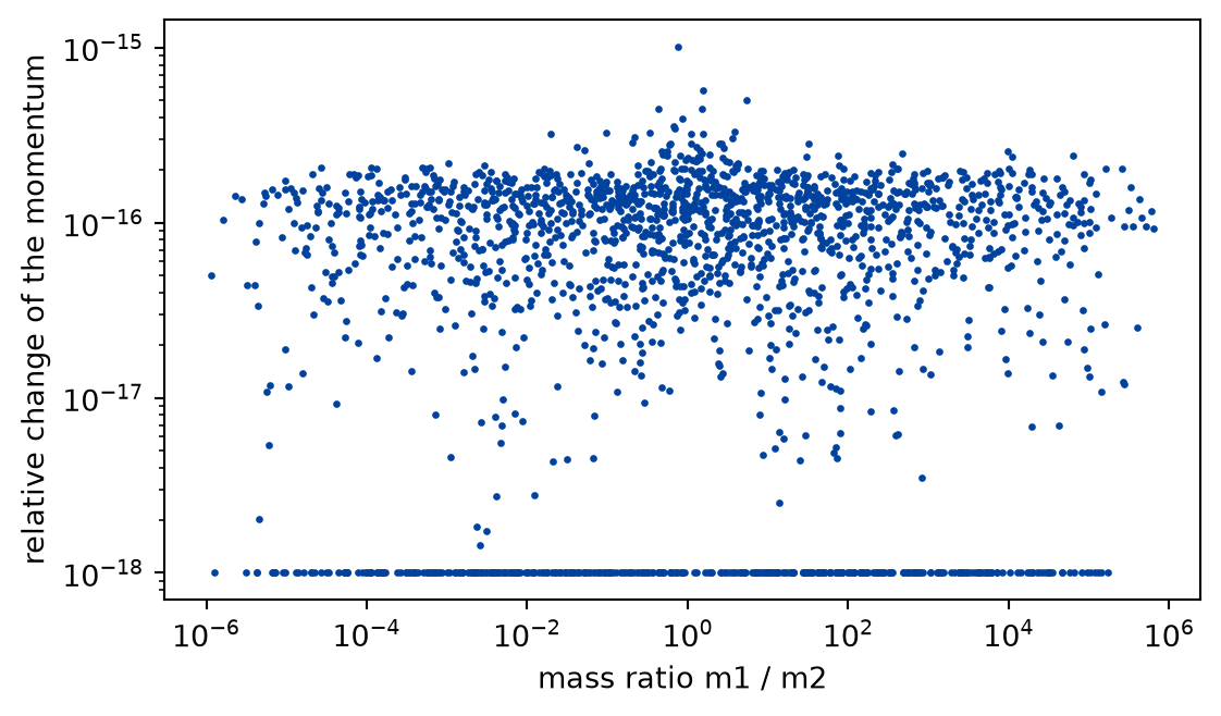
The same check over many more collisions, with the mass ratio over six orders of magnitude, shows what the table suggests.
def momentum_residuals(rng):"""The relative change of the momentum in two thousand collisions over six decades of the mass ratio, drawn from ``rng``.""" ratio, change = [], []for _ inrange(2000): mass_1, mass_2 =10** rng.uniform(-3, 3, size=2) velocity_1, velocity_2 = rng.normal(size=(2, 3)) normal = rng.normal(size=3) normal /= np.linalg.norm(normal) w1, w2 = hard_sphere_collision(mass_1, velocity_1, mass_2, velocity_2, normal) before = mass_1 * velocity_1 + mass_2 * velocity_2 ratio.append(mass_1 / mass_2) change.append( np.linalg.norm(mass_1 * w1 + mass_2 * w2 - before) / np.linalg.norm(before) )return ratio, change
def draw_momentum_residual(ratio, change) -> Figure:"""The relative change of the momentum against the mass ratio.""" fig, ax = plt.subplots(figsize=(6.4, 3.6)) ax.loglog(ratio, np.maximum(change, 1e-18), ".", color="#00429d", markersize=3) ax.set_xlabel("mass ratio m1 / m2") ax.set_ylabel("relative change of the momentum")return fig
Figure 1: simulated Change of the total momentum, relative to its size, in two thousand random collisions against the mass ratio. The rule never changes it by more than round-off.
The points lie on a band at the level of double precision, and the band does not widen with the mass ratio: the cancellation of the theorem does not depend on the masses. Points at the bottom edge are collisions whose change was exactly zero.
A rule the theorem does not describe
The theorem is about this rule. Take a rule that is almost the same, with the coefficient of an equal-mass collision used for unequal masses: both spheres change velocity by the same amount along , in opposite directions. Every part of the statement still looks plausible. The cell shows that the momentum is not conserved.
def two_rules(experiment: Experiment):"""Exercise 1: the change of the momentum with equal coefficients and with the rule of the momentum lesson; record the table and return the velocities after the right rule.""" approach = (v1 - v2) @ n wrong = (v1 - approach * n, v2 + approach * n) # coefficient 1 for any masses right = hard_sphere_collision(m1, v1, m2, v2, n) before = m1 * v1 + m2 * v2 rule_rows = [ ("rule with equal coefficients", *(m1 * wrong[0] + m2 * wrong[1] - before)), ("rule of the momentum lesson", *(m1 * right[0] + m2 * right[1] - before)), ] experiment.table("two-rules", rule_rows, [ ("rule", "", ""), ("x", "kg m/s", ".1e"), ("y", "kg m/s", ".1e"), ("z", "kg m/s", ".1e"), ],"The change of the total momentum along each axis, for two rules.", )return right
The change of the total momentum along each axis, for two rules.
rule
x (kg m/s)
y (kg m/s)
z (kg m/s)
rule with equal coefficients
6.0e+00
0.0e+00
0.0e+00
rule of the momentum lesson
0.0e+00
0.0e+00
0.0e+00
The first rule changes the momentum along the line of contact. It fails the proof at the place where the coefficients and cancel, which is exactly the algebra that ring checks in the theorem.
Limits
Momentum only. The theorem says nothing about the kinetic energy. That the rule conserves it for a unit direction n is a second theorem, not proved here. A rule can conserve momentum and lose energy, as an inelastic collision does.
The rule, not the force. The theorem takes the velocities after the collision from the rule. It does not derive the rule from forces, and it does not cover the soft contact that the simulation of the momentum lesson integrates; that conserves momentum for another reason, the equal and opposite forces of the pair, which is a statement about a sum over steps.
The Python code. Nothing here is a statement about pbc.mechanics. That the program implements the rule is what its unit tests and the table above check, for the cases they run.
Floating-point arithmetic.ℝ is exact; a double has a relative error of about one part in per operation, and the theorem does not speak about it.
More than two bodies. The statement is about one pair. A gas of many spheres is a sequence of pair collisions, and an induction over it is not proved here.
Self-check. The theorem holds for every direction n, including one of length two. Does the rule then describe a physical collision for such an n?
With scripts, you can record in this browser that you answered this question.
Solution to the self-check
No. The theorem only uses the shape of the rule: the two changes are multiples of the same vector with opposite signs and masses that cancel. A direction of length two makes the rule reverse the relative velocity along it by more than the factor that conserves the kinetic energy, so the collision creates or destroys energy, while the momentum stays. Conservation of momentum alone does not make a collision elastic.
Exercises
Exercise 1.Which hypotheses can go? The theorem needs hm₁ and hm₂. Which of them does the proof use, and where? What happens to the rule if ?
Solution to exercise 1
Neither positivity is used on its own: the proof needs only that , which is what hM states, and the two positive masses give it. If the masses summed to zero, Lean’s division by zero would make both coefficients zero, the rule would leave both velocities as they are, and momentum would be conserved for a trivial reason. A formal statement can hold for a reason that has nothing to do with the physics, which is why the hypotheses are stated and not only the conclusion. The physics needs positive masses anyway.
def total_mass():"""Exercise 2: the total mass the rule divides by.""" total = m1 + m2print(f"the rule divides by m1 + m2 = {total:.1f} kg for the example masses")
the rule divides by m1 + m2 = 4.0 kg for the example masses
Exercise 2.The centre of mass. The centre-of-mass velocity of the pair is . What does the theorem say about it, and which Lean statement would you write?
Solution to exercise 2
It is the same before and after, because the numerator is the total momentum and the denominator does not change. In Lean the statement is (m₁ * firstAfter m₁ m₂ v₁ v₂ n i + m₂ * secondAfter m₁ m₂ v₁ v₂ n i) / (m₁ + m₂) equal to the same expression with v₁ i and v₂ i, and the proof is collision_momentum followed by congrArg.
def centre_of_mass_velocity(right):"""Exercise 3: the change of the velocity of the centre of mass.""" w1, w2 = right centre_before = (m1 * v1 + m2 * v2) / (m1 + m2) centre_after = (m1 * w1 + m2 * w2) / (m1 + m2)print("largest change of the centre-of-mass velocity: "f"{np.max(np.abs(centre_after - centre_before)):.1e} m/s" )
The experiment writes every figure of this page into results/, as <label>.png, and every number and table of the page, as the page shows it, into results/results.json. Its numbers match this page to the digits shown, and its figure files are the ones the page shows; digits beyond those can differ between machines, because floating-point libraries differ. Change the code of the experiment and run it again to see what changes.
lake build compiles the proofs of this page with the Lean toolchain that elan installs; the first run fetches the Mathlib build cache, which is large. The setup page says how to install elan.