What symplectic Euler conserves

A modified energy that every step of symplectic Euler leaves exactly unchanged on the harmonic oscillator, stated and proved in Lean 4, with the step size under which it stays bounded, and the reason the energy of the method oscillates and does not grow.

Course

Classical mechanics, lesson 26 of 28

Methods

Formal proofs

Difficulty

Advanced, level 3 of 3

What you’ll learn

State the modified energy of symplectic Euler and its conservation as theorems in Lean 4
Read the proof by induction that the modified energy is the same after any number of steps
Say what the theorem explains about the bounded energy seen in the simulation, and what it does not prove

Prerequisites

Numerical integrators, Proving what the simulation showed.

Before you begin

Algebra: completing the square in two variables

Related

none

Previous

Momentum in a collision, proved

Next

Lean exercises on your machine

With scripts, this page keeps a record in your browser of whether you completed the lesson. Nothing is stored without them.

With scripts, this place suggests what to do next, with the reason, from the progress saved in your browser. Without them, follow the learning path.

The numerical integrators lesson found that symplectic Euler does what explicit Euler cannot: on the harmonic oscillator its energy does not drift away. It swings a little above and below its starting value, over and over, for as long as the run lasts. The first Lean lesson proved the opposite for explicit Euler, a factor greater than one at every step. A run shows the bounded energy of symplectic Euler for the step sizes it was given and not for any other, and it does not say why.

The reason is a quantity that each step of symplectic Euler leaves exactly where it was. It is not the energy of the spring but a neighbour of it: the energy minus a small term. This lesson states that quantity in Lean and proves that it is conserved, for any state and any step size, and then proves that it is not negative when the step is small. The energy of the spring differs from it by a term that stays small, which is the oscillation the simulation shows.

Assumptions

Every assumption of the model is a hypothesis of a theorem or a definition; the build fails on sorry and on any axiom the project declares.

Newton’s second law with Hooke’s law. The mass $m$ on a spring $k$ accelerates as $m\,a = -k\,x$ : the hypothesis hnewton.
The update rule of symplectic Euler. The velocity changes first, with the acceleration at the old position (hv'), and the particle moves with the new velocity (hx'). Moving with the old velocity is explicit Euler, which the first Lean lesson covers and which has no such conserved quantity.
A positive mass. hm : 0 < m lets the proof divide by the mass.
For the bound: a spring that pulls back, and a small step. The non-negativity of the modified energy needs hk : 0 < k and hdt : k * dt ^ 2 < 4 * m. The condition says that the step is shorter than a fraction of the period; for a longer step the quantity is still conserved but can be negative, and the bound is lost.
Real numbers, not floating-point numbers. Lean’s ℝ has no round-off. The program computes with doubles, and the conservation holds for them only up to the round-off of every step.
No derivatives. The facts are algebraic. The theorem does not mention the motion in continuous time, and it does not say how close the modified energy is to the true one.

What the theorems say

Write $\omega^2 = k/m$ for the squared angular frequency. One step of symplectic Euler is

$v' = v - \omega^2\,x\,\Delta t, \qquad x' = x + \Delta t\,v'.$

The energy of the spring is $E = \tfrac12 m v^2 + \tfrac12 k x^2$ . The modified energy subtracts a cross term:

$\tilde E = E - \tfrac12\,k\,\Delta t\,x\,v.$

One step leaves $\tilde E$ unchanged. The proof expands the two sides in $x$ and $v$ and compares them: the terms in $x v$ that the new velocity inside the position update introduces are exactly what the cross term removes.

Formal theorem (symplectic Euler on a mass of positive mass on a spring, any step size, real arithmetic): One step of symplectic Euler on the harmonic oscillator leaves the modified energy unchanged.

Formal theorem (symplectic Euler on the oscillator, any step size and any number of steps, real arithmetic): After any number of steps of symplectic Euler, the modified energy equals its initial value.

Formal theorem (the step sizes below the stated limit, real arithmetic): For a spring constant that is positive and a step with $k\,\Delta t^2 < 4m$ , the modified energy is never negative.

The third statement is what turns a conserved number into a bound. With a non-negative conserved quantity of this shape, the motion stays inside an ellipse in $(x, v)$ : position and velocity cannot grow without limit. The cross term is small when the step is small, so the true energy stays near the modified one, and the simulation sees it oscillate.

The proofs

The listings are read from the Lean files of the repository when the site is built, and they are the text that lake build compiled.

Compiled with Lean 4.34.1 and Mathlib v4.34.1: ./scripts/check-lean.sh found no sorry and no axiom declared by the project before this page was built.

Commit 6417e2ff90258bd2d2ba21d217eb7666fd24f680 of the repository.

What was checked, and where to read the proofs

./scripts/check-lean.sh ran lake build on every module of the project and found no sorry and no axiom declared by the project before this page was built. CI runs the same check on every pull request and on main.

Lean 4.34.1, from the toolchain pinned in lean/lean-toolchain.
Mathlib v4.34.1, revision d13f23b723.
lean/PhysicsByConstruction/Mechanics/SymplecticEuler.lean, or open it in the Lean web editor

The file in the repository at that commit and the result of the CI run are authoritative. The Lean web editor is a convenience: it runs its own version of Mathlib, which can differ from the one above, so a proof that compiled here may report an error there.

The definition. It reuses springEnergy from the first Lean lesson’s file and subtracts the cross term.

/-- The modified energy of symplectic Euler with the time step `dt`: the
energy of the spring minus `k dt x v / 2`. -/
noncomputable def modifiedEnergy (m k dt x v : ℝ) : ℝ :=
  springEnergy m k x v - k * dt * x * v / 2

lean/PhysicsByConstruction/Mechanics/SymplecticEuler.lean, lines 24 to 27, read from the repository when this page was built.

One step. The hypotheses hv' and hx' are the update rule, and hnewton is the law of the spring. Compare hx' here with the one of explicit Euler: the position uses v'.

/-- **One symplectic Euler step leaves the modified energy unchanged.**

`hv'` updates the velocity with the acceleration at the old position, and
`hx'` moves the particle with the *new* velocity. `hnewton` is Newton's law
for the spring, `m a = -k x`. -/
theorem symplectic_modified_energy_step
    (m k x v a dt x' v' : ℝ) (hm : 0 < m)
    (hnewton : m * a = -k * x)
    (hv' : v' = v + dt * a)
    (hx' : x' = x + dt * v') :
    modifiedEnergy m k dt x' v' = modifiedEnergy m k dt x v := by
  have ha : a = -k * x / m := by
    field_simp
    linarith [mul_comm m a]
  subst hx' hv' ha
  unfold modifiedEnergy springEnergy
  field_simp
  ring

lean/PhysicsByConstruction/Mechanics/SymplecticEuler.lean, lines 31 to 48, read from the repository when this page was built.

Any number of steps, by induction. The base case is the initial state. The step rewrites the energy after one more step with the one-step theorem, then uses the hypothesis of the induction.

/-- **After any number of steps the modified energy is the initial one.**
By induction on the number of steps, from the one-step theorem. -/
theorem symplectic_modified_energy_after_steps
    (m k dt : ℝ) (hm : 0 < m) (x v a : ℕ → ℝ)
    (hnewton : ∀ n, m * a n = -k * x n)
    (hv : ∀ n, v (n + 1) = v n + dt * a n)
    (hx : ∀ n, x (n + 1) = x n + dt * v (n + 1)) (n : ℕ) :
    modifiedEnergy m k dt (x n) (v n) = modifiedEnergy m k dt (x 0) (v 0) := by
  induction n with
  | zero => rfl
  | succ n ih =>
    rw [symplectic_modified_energy_step m k (x n) (v n) (a n) dt _ _ hm
      (hnewton n) (hv n) (hx n), ih]

lean/PhysicsByConstruction/Mechanics/SymplecticEuler.lean, lines 52 to 64, read from the repository when this page was built.

The bound. The proof completes a square: the quadratic form in $x$ and $v$ is a square plus a positive multiple of $x^2$ whenever the step is short.

/-- **The modified energy is not negative when the step is small.** For
`k Δt² < 4 m` the quadratic form `m v² - k Δt x v + k x²` has no negative
value, so the conserved quantity bounds the motion: `x` and `v` cannot grow
without limit. -/
theorem modified_energy_nonneg
    (m k dt x v : ℝ) (hm : 0 < m) (hk : 0 < k) (hdt : k * dt ^ 2 < 4 * m) :
    0 ≤ modifiedEnergy m k dt x v := by
  unfold modifiedEnergy springEnergy
  have h1 : 0 ≤ (m * v - k * dt * x / 2) ^ 2 := sq_nonneg _
  have h2 : 0 ≤ k * (4 * m - k * dt ^ 2) * x ^ 2 := by
    have : 0 < 4 * m - k * dt ^ 2 := by linarith
    positivity
  have h3 : 0 ≤ m * (m * v ^ 2 / 2 + k * x ^ 2 / 2 - k * dt * x * v / 2) := by
    nlinarith
  exact nonneg_of_mul_nonneg_right h3 hm

lean/PhysicsByConstruction/Mechanics/SymplecticEuler.lean, lines 68 to 82, read from the repository when this page was built.

Worked examples

The conserved quantity in a run

Half a kilogram on a spring of two newtons per metre, pulled out one metre and released, run with symplectic Euler for three periods at sixteen steps per period. The cell measures the energy of the spring and the modified energy along the run.

mass = 0.5  # kg
k = 2.0  # N/m
period = 2 * np.pi / angular_frequency(mass, k)
steps_per_period = 16
dt = period / steps_per_period
n_steps = 3 * steps_per_period

src/pbc/mechanics/experiments/symplectic_euler_conserved_energy.py, lines 26 to 31, read from the repository when this page was built.

def modified_energy(trajectory):
    """The energy of the spring minus k dt x v / 2, at every instant (J)."""
    cross = np.sum(trajectory.x * trajectory.v, axis=1)
    return energy(trajectory, mass, k) - 0.5 * k * dt * cross

src/pbc/mechanics/experiments/symplectic_euler_conserved_energy.py, lines 35 to 38, read from the repository when this page was built.

def three_periods(experiment: Experiment):
    """Three periods with symplectic Euler: the energy of the spring and the
    modified energy; record the table."""
    symplectic = simulate(
        State(t=0.0, x=1.0, v=0.0),
        newton(mass, spring(k)),
        dt,
        n_steps,
        step=symplectic_euler_step,
    )
    spring_energy = energy(symplectic, mass, k)
    modified = modified_energy(symplectic)
    drift = np.max(np.abs(modified / modified[0] - 1))
    swing = spring_energy.max() / spring_energy.min() - 1

    experiment.table(
        "three-periods",
        [
            ("energy of the spring", spring_energy.min(), spring_energy.max()),
            ("modified energy", modified.min(), modified.max()),
        ],
        [("quantity", "", ""), ("smallest", "J", ".4f"), ("largest", "J", ".4f")],
        "The energy of the spring and the modified energy over the run, symplectic "
        "Euler.",
    )
    return symplectic, spring_energy, modified, drift, swing

src/pbc/mechanics/experiments/symplectic_euler_conserved_energy.py, lines 41 to 66, read from the repository when this page was built.

The energy of the spring and the modified energy over the run, symplectic Euler.
quantity	smallest (J)	largest (J)
energy of the spring	0.8403	1.2390
modified energy	1.0000	1.0000

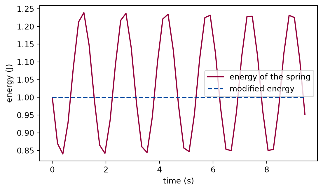
The modified energy is the same at every step to round-off (the relative change over the run is 8e-16), while the energy of the spring swings by a relative 0.47 between its smallest and largest value. That is the theorem on a run, and the swing is the cross term at work.

def draw_modified_energy(symplectic, spring_energy, modified) -> Figure:
    """The energy of the spring and the modified energy against time."""
    fig, ax = plt.subplots(figsize=(6.4, 3.6))
    ax.plot(symplectic.t, spring_energy, color="#93003a", label="energy of the spring")
    ax.plot(
        symplectic.t, modified, color="#00429d", linestyle="--", label="modified energy"
    )
    ax.set_xlabel("time (s)")
    ax.set_ylabel("energy (J)")
    ax.legend()
    return fig

src/pbc/mechanics/experiments/symplectic_euler_conserved_energy.py, lines 69 to 79, read from the repository when this page was built.

Plot of energy in joules against time in seconds over three periods. One curve, the energy of the spring, oscillates up and down with the period of the motion. A second curve, the modified energy, is a flat horizontal line. — Figure 1: simulated The energy of the spring swings above and below its start under symplectic Euler, while the modified energy stays on the line.

The same quantity under explicit Euler

The theorem is about the rule of symplectic Euler. Under explicit Euler the same quantity, and the energy of the spring too, are not conserved.

def explicit_euler():
    """Exercise 1: the modified energy along explicit Euler."""
    explicit = simulate(
        State(t=0.0, x=1.0, v=0.0),
        newton(mass, spring(k)),
        dt,
        n_steps,
        step=euler_step,
    )
    explicit_modified = modified_energy(explicit)
    growth = explicit_modified[-1] / explicit_modified[0]
    print(
        "modified energy after three periods of explicit Euler, relative to the"
        f" start: {growth:.2f}"
    )

src/pbc/mechanics/experiments/symplectic_euler_conserved_energy.py, lines 82 to 96, read from the repository when this page was built.

modified energy after three periods of explicit Euler, relative to the start: 788.88

The modified energy of explicit Euler grows with the energy. The quantity is a property of the update rule and not of the oscillator alone.

The bound and the step size

The bound needs $k\,\Delta t^2 < 4m$ , that is, a step shorter than the period divided by $\pi$ . Above it the quadratic form is indefinite. The cell evaluates the smallest value of the modified energy over the unit circle in $(x, v)$ for several step sizes.

def positive_or_not(experiment: Experiment) -> None:
    """Exercise 2: the smallest modified energy on the unit circle for four
    steps; record the table."""
    angles = np.linspace(0, 2 * np.pi, 3601)
    rows = []
    for per_period in (64, 16, 4, 3):
        step = period / per_period
        x, v = np.cos(angles), np.sin(angles)
        value = 0.5 * mass * v**2 + 0.5 * k * x**2 - 0.5 * k * step * x * v
        rows.append((per_period, k * step**2 / (4 * mass), value.min()))

    experiment.table(
        "positive-or-not",
        rows,
        [
            ("steps per period", "", "d"),
            ("k dt^2 / 4m", "", ".3f"),
            ("smallest modified energy on the circle", "J", ".4f"),
        ],
        "The smallest value of the modified energy on the unit circle in position "
        "and velocity, for four step sizes.",
    )

src/pbc/mechanics/experiments/symplectic_euler_conserved_energy.py, lines 99 to 120, read from the repository when this page was built.

The smallest value of the modified energy on the unit circle in position and velocity, for four step sizes.
steps per period	k dt^2 / 4m	smallest modified energy on the circle (J)
64	0.002	0.2492
16	0.039	0.2374
4	0.617	0.0820
3	1.097	-0.0190

While the ratio $k\,\Delta t^2/4m$ is below one the minimum is positive, which is the theorem. The last row has a ratio above one, and its minimum is no longer positive: the bound is lost there.

Limits

A statement about the method, not the physics. The modified energy is conserved by the update rule. That the energy of the spring stays near it is what the cross term, small for a small step, says, and it is an estimate that is not proved here.
Only the harmonic oscillator. The conserved quantity was found for the linear force of a spring. For other forces, symplectic methods conserve a modified energy only approximately, a result that needs more than algebra.
The Python code. Nothing here is a statement about pbc.mechanics. The theorem is about the rule written in Lean; the table above checks, for one run, that the program follows it.
Floating-point arithmetic. ℝ is exact. A double carries a rounding error in every step, and the modified energy of a long run of the program drifts by a random walk of those errors.
Stability of the method. The bound is on the quantity. A step that violates hdt is not shown unstable by this lesson, only left without the bound.

Self-check. The theorem says the modified energy is the same after every step. Why does the ordinary energy of the spring still change?

With scripts, you can record in this browser that you answered this question.

Solution to the self-check

Because the conserved quantity is the energy plus a cross term $-\tfrac12 k\,\Delta t\,x\,v$ that changes during the oscillation: it is positive when the particle moves away from the centre and negative when it returns. The sum is constant, so the energy of the spring changes by the opposite of the cross term, which is bounded and small for a small step.

Exercises

Exercise 1. Why the cross term? Suppose the conserved quantity had the form $\tfrac12 m v^2 + \tfrac12 k x^2 + c\,x v$ for some constant $c$ . Find $c$ so that the coefficient of $v'^2$ after a step is again $\tfrac12 m$ .

Solution to exercise 1

After one step the quantity is $\tfrac12 m v'^2 + \tfrac12 k x'^2 + c\,x' v'$ with $x' = x + \Delta t\,v'$ . Collecting the coefficient of $v'^2$ gives $\tfrac12 m + \tfrac12 k\,\Delta t^2 + c\,\Delta t$ , which equals $\tfrac12 m$ only for $c = -\tfrac12 k\,\Delta t$ . The coefficient of $x v'$ is then $\tfrac12 k\,\Delta t$ , and substituting $v' = v - (k/m)\,x\,\Delta t$ turns the whole expression back into the quantity before the step. The cell checks it on a random state.

def quantity(x, v, c):
    return 0.5 * mass * v**2 + 0.5 * k * x**2 + c * x * v

src/pbc/mechanics/experiments/symplectic_euler_conserved_energy.py, lines 123 to 124, read from the repository when this page was built.

def the_value_of_c():
    """Exercise 3: the value of c, checked on a random state."""
    rng = np.random.default_rng(3)
    x0, v0 = rng.normal(size=2)
    v1 = v0 - k / mass * x0 * dt
    x1 = x0 + dt * v1
    c = -0.5 * k * dt
    print(
        "change of the quantity over a step with c = -k dt / 2: "
        f"{quantity(x1, v1, c) - quantity(x0, v0, c):.1e}"
    )

src/pbc/mechanics/experiments/symplectic_euler_conserved_energy.py, lines 127 to 137, read from the repository when this page was built.

change of the quantity over a step with c = -k dt / 2: -1.8e-15

Exercise 2. How many steps per period? The bound needs $k\,\Delta t^2 < 4m$ . How many steps per period is that, at least?

Solution to exercise 2

With $\Delta t = T/N$ and $T = 2\pi/\omega$ , the condition $\omega^2\Delta t^2 < 4$ reads $N > \pi$ , so four steps per period are enough and three are not, however large $m$ and $k$ are.

def fewest_steps():
    """Exercise 4: the bound on the steps per period."""
    print(f"pi = {np.pi:.4f}: the number of steps per period must exceed it")

src/pbc/mechanics/experiments/symplectic_euler_conserved_energy.py, lines 140 to 142, read from the repository when this page was built.

pi = 3.1416: the number of steps per period must exceed it

Check this proof

This page was built from commit 6417e2ff90258bd2d2ba21d217eb7666fd24f680 of the repository.

In a clone at that commit, with the pinned Lean toolchain, this command in lean/ checks the proofs of this page:

lake build PhysicsByConstruction.Mechanics.SymplecticEuler

Files, tests, and every command

The files behind it:

site/lessons/lean/03-what-symplectic-euler-conserves/index.qmd: this page, with every code cell.
lean/PhysicsByConstruction/Mechanics/EulerOscillator.lean: a Lean file the page shows.
lean/PhysicsByConstruction/Mechanics/SymplecticEuler.lean: a Lean file the page shows.
src/pbc/mechanics/integrators.py: code the experiment runs.
src/pbc/mechanics/oscillator.py: code the experiment runs.
src/pbc/mechanics/experiments/symplectic_euler_conserved_energy.py: code the experiment runs.
src/pbc/experiment.py: code the experiment runs.
tests/unit/test_integrators.py: tests of that code.
tests/unit/test_oscillator.py: tests of that code.
tests/unit/test_symplectic_euler_conserved_energy_experiment.py: tests of that code.

With Git and uv, and elan for the proofs, installed (see the setup page), run:

git clone https://github.com/taspinar/physics-by-construction.git
cd physics-by-construction
git checkout 6417e2ff90258bd2d2ba21d217eb7666fd24f680
uv sync --locked --no-dev
uv run --locked --no-dev python -m pbc.mechanics.experiments.symplectic_euler_conserved_energy results
cd lean
lake exe cache get
lake build PhysicsByConstruction.Mechanics.SymplecticEuler

The experiment writes every figure of this page into results/, as <label>.png, and every number and table of the page, as the page shows it, into results/results.json. Its numbers match this page to the digits shown, and its figure files are the ones the page shows; digits beyond those can differ between machines, because floating-point libraries differ. Change the code of the experiment and run it again to see what changes.

lake build compiles the proofs of this page with the Lean toolchain that elan installs; the first run fetches the Mathlib build cache, which is large. The setup page says how to install elan.