The Kepler orbit

The physics capstone of the mechanics course: two bodies under gravity reduced to one, the energy and the angular momentum that fix the ellipse, the exact orbit to measure against, and what each integrator does to a thousand orbits, with every tool of the earlier lessons reused.

Course

Classical mechanics, lesson 8 of 28

Slot

M8, Kepler orbits

Methods

Simulation

Difficulty

Advanced, level 3 of 3

What you’ll learn

• Reduce two bodies under gravity to one
• Derive the ellipse, its size, and its period from the energy and the angular momentum
• Compare each integrator with the exact orbit over a thousand orbits

Prerequisites

Energy conservation, Momentum and collisions.

Before you begin

• Vectors: the cross product in three dimensions, and the identity a × (b × c) = b (a·c) − c (a·b)
• Geometry: the ellipse, its foci, semi-major axis, and eccentricity
• Numerical methods: the Newton iteration for the root of an equation

Related

Gravitational-wave strain lab

Previous

Momentum and collisions

Next

Verifying scientific code

With scripts, this page keeps a record in your browser of whether you completed the lesson. Nothing is stored without them.

With scripts, this place suggests what to do next, with the reason, from the progress saved in your browser. Without them, follow the learning path.

The Earth returns to the same point of its path once a year, and has done so for as long as anyone has recorded it. Why does the path close at all? A force that depends on the distance alone could just as well send a planet spiralling in or out. And once a computer is asked to follow the planet, a second question appears: for how many orbits does a simulation keep the planet on the ellipse it started on? Neither question needs a new idea of mechanics. Two bodies attract each other with a pairwise force, and the momentum lesson turns them into one body about a fixed centre. The force is conservative, so the energy of the energy lesson is conserved; it is central, so the angular momentum is conserved too. The two constants fix the size and the shape of the orbit before anything is simulated, and an equation Kepler wrote down gives the exact motion to compare with, as the cosine did for the oscillator.

The simulation then uses the four integrators of the course on this force and asks the question that was asked of each earlier system, now for the long run. One orbit is easy. A thousand orbits separate the methods completely: one keeps the energy in a band and the angular momentum to round-off while the ellipse slowly turns; another follows the planet more closely for a year and loses it within a century. The lesson ends with the two bodies simulated as two bodies, the star wobbling about the common centre of mass at a speed that is how planets around other stars are found.

Assumptions

The model and the program rest on these assumptions. Each one names what goes wrong when it does not hold.

1. Two bodies and nothing else. A third body makes the problem non-integrable: in general no fixed Keplerian ellipse, no closed-form solution to compare with, and over long times chaotic sensitivity to the initial state (special periodic solutions exist, but not as a general rule). The methods and diagnostics of this lesson still apply, the exact reference does not.
2. Point masses under Newtonian gravity. The bodies are spheres small compared with their distance, or spherically symmetric, so each attracts as a point. Tides, the oblateness of a star, and general relativity add small forces that make the real perihelion of a planet precess; the precession the simulation shows below is not one of them but an error of the method, and the lesson says how to tell.
3. Motion in a plane. Two bodies always move in the plane that holds their relative position and velocity, so two coordinates suffice, and the angular momentum is one number, the component perpendicular to the plane.
4. A bound orbit. The energy is negative, the orbit is an ellipse and repeats. At or above the escape speed the motion is a parabola or a hyperbola, orbital_elements reports that the orbit is not bound, and the second exercise shows both sides of the line. A body that moves straight at the centre has no angular momentum and no ellipse either, and the code refuses it.
5. A step that is a fraction of the orbit. The steps per orbit are chosen for the fast passage through the perihelion; at the aphelion the same step is finer than needed. An eccentric orbit wastes most of its steps that way, and a method that adapts the step is the usual remedy and beyond this course.
6. Astronomical units. Distances are in astronomical units, times in years, and masses in solar masses. The value $GM = 4\pi^2$ in these units is not a measurement but a choice that follows from Kepler’s third law below: it makes an orbit with a semi-major axis of one astronomical unit last exactly one year. Speeds in metres per second convert the unit with the SI astronomical unit and the Julian year of scipy.constants. The functions take $G$ or $GM$ as an argument, so nothing in the code depends on the choice.
7. One orbit and one step for the long-run results. The thousand-orbit results are for an eccentricity of one half and a hundred steps per orbit; the lesson varies the step, not the eccentricity, and states nothing about other eccentricities beyond what the derivations say.
8. Round-off is negligible. The conserved quantities of the symplectic methods stay at the level of double-precision round-off, far below every other quantity on the page; the tables show such a value as a bound, not as a number.

Two bodies, one orbit

The reduction to one body

Two bodies of masses $m_1$ and $m_2$ attract each other along the line between them with the force $G m_1 m_2 / r^2$, where $r$ is their distance. On the first body, at the position $\mathbf r = \mathbf x_1 - \mathbf x_2$ relative to the second, the force is

$$\mathbf F = -\,\frac{G\,m_1 m_2}{r^3}\,\mathbf r ,$$

and the second body feels $-\mathbf F$. The accelerations are $\ddot{\mathbf x}_1 = \mathbf F / m_1$ and $\ddot{\mathbf x}_2 = -\mathbf F / m_2$, so the relative position obeys

$$\ddot{\mathbf r} = \ddot{\mathbf x}_1 - \ddot{\mathbf x}_2 = \Bigl(\frac{1}{m_1} + \frac{1}{m_2}\Bigr)\mathbf F = \frac{\mathbf F}{\mu}, \qquad \frac{1}{\mu} = \frac{1}{m_1} + \frac{1}{m_2},$$

with the reduced mass $\mu$ of the momentum lesson. Since $m_1 m_2 / \mu = m_1 + m_2 = M$, the factor $\mu$ cancels the product of the masses and

$$\ddot{\mathbf r} = -\,\frac{GM}{r^3}\,\mathbf r .$$

The two-body problem is a one-body problem: a particle at $\mathbf r$ about a fixed centre with the gravitational parameter $GM$. The momentum lesson showed that the centre of mass $\mathbf X$ moves in a straight line, and the position of each body follows from $\mathbf r$ and $\mathbf X$: $\mathbf x_1 = \mathbf X + \tfrac{m_2}{M}\mathbf r$ and $\mathbf x_2 = \mathbf X - \tfrac{m_1}{M}\mathbf r$. For a planet about a star $M$ is the star’s mass to a part in a thousand at most, and the planet’s own mass enters the orbit only through that small correction, which is why Kepler’s laws hold for every planet alike.

Two conserved quantities

The force is conservative, with the potential energy $-GM\mu/r$, zero at infinite separation. Per unit mass the energy of the relative motion is $\varepsilon = \tfrac12 |\mathbf v|^2 - GM/r$, with $\mathbf v = \dot{\mathbf r}$, and it is constant because its rate of change vanishes:

$$\dot\varepsilon = \mathbf v\cdot\dot{\mathbf v} + \frac{GM}{r^3}\,\mathbf r\cdot\mathbf v = -\frac{GM}{r^3}\,\mathbf v\cdot\mathbf r + \frac{GM}{r^3}\,\mathbf r\cdot\mathbf v = 0 .$$

The force is also central, directed along $\mathbf r$, and a central force exerts no torque about the centre. The angular momentum per unit mass $\mathbf h = \mathbf r \times \mathbf v$ has the rate of change $\mathbf v \times \mathbf v + \mathbf r \times \dot{\mathbf v}$, and both cross products are of parallel vectors: $\mathbf h$ is constant. In the plane it is the single number $h = x\,v_y - y\,v_x$. The area swept out by the line from the centre grows at the rate $h/2$ (half the area of the parallelogram that $\mathbf r\,dt$ and $\mathbf v\,dt$ span), so a constant $h$ is Kepler’s second law. The angular momentum of the code is $L = \mu h$.

The shape of the orbit, derived

A third constant gives the shape. Differentiate $\mathbf v \times \mathbf h$, using that $\mathbf h$ is constant and the identity for a triple product:

$$\frac{d}{dt}\,(\mathbf v \times \mathbf h) = \dot{\mathbf v} \times (\mathbf r \times \mathbf v) = -\frac{GM}{r^3}\bigl(\mathbf r\,(\mathbf r\cdot\mathbf v) - \mathbf v\,r^2\bigr) = GM\Bigl(\frac{\mathbf v}{r} - \frac{\mathbf r\,(\mathbf r\cdot\mathbf v)}{r^3}\Bigr) = GM\,\frac{d}{dt}\frac{\mathbf r}{r} .$$

So $\mathbf v\times\mathbf h - GM\,\mathbf r/r$ is constant. Written as a dimensionless vector, this is the eccentricity vector

$$\mathbf e = \frac{\mathbf v \times \mathbf h}{GM} - \frac{\mathbf r}{r} = \frac{|\mathbf v|^2\,\mathbf r - (\mathbf r\cdot\mathbf v)\,\mathbf v}{GM} - \frac{\mathbf r}{r},$$

and $e = |\mathbf e|$ is the eccentricity. Take the dot product with $\mathbf r$, and use $\mathbf r\cdot(\mathbf v\times\mathbf h) = \mathbf h\cdot(\mathbf r\times\mathbf v) = h^2$:

$$\mathbf e\cdot\mathbf r = \frac{h^2}{GM} - r \quad\Longrightarrow\quad r = \frac{h^2 / GM}{1 + e\cos\theta},$$

where $\theta$ is the angle from $\mathbf e$ to $\mathbf r$. This is the polar equation of a conic with a focus at the centre, and it is an ellipse exactly when $e < 1$: Kepler’s first law. The closest point is at $\theta = 0$, in the direction of $\mathbf e$, so the eccentricity vector points from the centre to the perihelion, and the farthest at $\theta = \pi$. The two distances are $a(1-e)$ and $a(1+e)$ for the semi-major axis $a$, so their sum is $2a$:

$$2a = \frac{h^2}{GM}\Bigl(\frac{1}{1+e} + \frac{1}{1-e}\Bigr) = \frac{2h^2}{GM\,(1-e^2)} .$$

The size of $\mathbf e$ follows from squaring its definition, with $|\mathbf v\times\mathbf h|^2 = |\mathbf v|^2 h^2$ (the two are perpendicular) and the same dot product once more:

$$e^2 = \frac{|\mathbf v|^2 h^2}{(GM)^2} - \frac{2h^2}{GM\,r} + 1 = 1 + \frac{2\,\varepsilon\,h^2}{(GM)^2} ,$$

so $e < 1$ is the same statement as $\varepsilon < 0$: a bound orbit is an ellipse. Putting $1 - e^2 = -2\varepsilon h^2/(GM)^2$ into the expression for $a$ gives the elements of the orbit in terms of the two constants,

$$a = -\,\frac{GM}{2\varepsilon}, \qquad e = \sqrt{1 + \frac{2\,\varepsilon\,h^2}{(GM)^2}}, \qquad T = 2\pi\sqrt{\frac{a^3}{GM}} .$$

The period is the area of the ellipse divided by the rate $h/2$ at which it is swept out. The ellipse is a circle of radius $a$ squeezed in one direction by the factor $b/a$, with the semi-minor axis $b = a\sqrt{1-e^2}$, so its area is $\pi a b$ and, with $h^2 = GM\,a\,(1-e^2)$,

$$T = \frac{\pi a b}{h/2} = \frac{2\pi a^2\sqrt{1-e^2}}{\sqrt{GM\,a\,(1-e^2)}} = 2\pi\sqrt{\frac{a^3}{GM}} :$$

Kepler’s third law, $T^2 \propto a^3$, with a constant that depends on $M$ alone. The code evaluates the length of $\mathbf e$ rather than the square root above, because the two are equal in exact arithmetic but not in floating point near a circle. These formulas turn any state into the orbit through it, so a simulation can be asked at every step which ellipse it is on: the energy and the angular momentum are the two diagnostics of the earlier lessons at once, and the eccentricity vector adds the orientation of the ellipse. A perihelion and an aphelion are the names of the closest and farthest points of an orbit about the Sun.

The exact motion

Where the body is on its ellipse at a given time has no closed form, but it has an equation that can be solved to any precision. Describe the position by the eccentric anomaly $u$, the angle of the point on the circle that the ellipse was squeezed from. In the frame of the ellipse, with $\hat{\mathbf P}$ along the perihelion and $\hat{\mathbf Q}$ a quarter turn ahead,

$$\mathbf r = a\,(\cos u - e)\,\hat{\mathbf P} + b\sin u\,\hat{\mathbf Q}, \qquad r = a\,(1 - e\cos u),$$

(the second follows from the first by squaring). The area swept from the perihelion is that of the circular sector of radius $a$ at the centre, $\tfrac12 a^2 u$, less the triangle that the centre, the focus, and the point span, $\tfrac12 (ae)(a\sin u)$, all scaled by $b/a$: $\tfrac12 a b\,(u - e\sin u)$. If the body is at perihelion at $t_0$, this area equals $(h/2)(t - t_0)$ with $h = 2\pi a b/T = n\,a\,b$, which gives Kepler’s equation,

$$u - e\,\sin u = n\,(t - t_0) + \ell_0, \qquad n = \frac{2\pi}{T},$$

whose right side, the mean anomaly $\ell$, grows uniformly in time. For a perihelion start $\ell_0 = 0$; for an arbitrary starting state the area already swept at $t_0$ adds to the right side, and $\ell_0$ is the mean anomaly at the start. It is solved for $u$ by the Newton iteration. With $f(u) = u - e\sin u - \ell$ the derivative $f'(u) = 1 - e\cos u$ is at least $1 - e > 0$ for an ellipse, so $f$ increases steadily, has exactly one root, and the tangent never flattens. Differentiating the equation gives $\dot u = n/(1 - e\cos u)$, and the velocity follows from the position by the chain rule, $\mathbf v = \dot u\,d\mathbf r/du$, with $n a = \sqrt{GM/a}$. This is the role the cosine played for the oscillator: the exact state at any time, for the error of a simulation to be measured against. The code starts the iteration from a starting value of Danby (the mean anomaly plus a correction of $0.85\,e$), which converges in a few steps for the eccentricities of this lesson.

Go deeper: Kepler's equation (Wikipedia, Numerical approximation of inverse problem, Newton's method; derivation.)

How Kepler’s equation is solved numerically: the Newton iteration for $u$, the starting values that suit small and large eccentricities, and why it is unreliable at the parabolic limit. The lesson does not need it; its own starting value is not the one on that page.

What the integrators do to it

The gravitational force is smooth and conservative, so the four methods keep the orders the numerical integrators lesson measured, and the energy behaves as it did there: explicit Euler feeds it in, the classical Runge-Kutta method drains it slowly and steadily, the symplectic methods keep it in a band. The angular momentum is new, and here the symplectic methods do something exact. Symplectic Euler changes the velocity by $\Delta t\,\mathbf a(\mathbf r_n)$, which is parallel to $\mathbf r_n$, and then the position by $\Delta t\,\mathbf v_{n+1}$, which is parallel to $\mathbf v_{n+1}$:

$$\mathbf r_{n+1} \times \mathbf v_{n+1} = (\mathbf r_n + \Delta t\,\mathbf v_{n+1}) \times \mathbf v_{n+1} = \mathbf r_n \times \mathbf v_{n+1} = \mathbf r_n \times (\mathbf v_n + \Delta t\,\mathbf a(\mathbf r_n)) = \mathbf r_n \times \mathbf v_n .$$

The angular momentum is conserved exactly at every step, for every step size, for any central force. Velocity Verlet needs two more lines. Its new velocity is $\mathbf v_{n+1} = \mathbf v_n + \tfrac12\Delta t\,(\mathbf a_n + \mathbf a_{n+1})$ and its new position is $\mathbf r_{n+1} = \mathbf r_n + \Delta t\,(\mathbf v_n + \tfrac12\Delta t\,\mathbf a_n)$. Write $\mathbf w = \mathbf v_n + \tfrac12\Delta t\,\mathbf a_n$. The acceleration $\mathbf a_{n+1}$ is parallel to $\mathbf r_{n+1}$ and drops out of the cross product with it, and $\mathbf a_n$ is parallel to $\mathbf r_n$:

$$\mathbf r_{n+1} \times \mathbf v_{n+1} = \mathbf r_{n+1} \times \mathbf w = (\mathbf r_n + \Delta t\,\mathbf w) \times \mathbf w = \mathbf r_n \times \mathbf v_n + \tfrac12\Delta t\,\mathbf r_n \times \mathbf a_n = \mathbf r_n \times \mathbf v_n .$$

Explicit Euler and the classical Runge-Kutta method have no such property: their velocity change is not parallel to the position at which the position change is taken, and the angular momentum drifts. The worked examples check all four.

What the bounded energy and the exact angular momentum do not fix is the orientation of the ellipse. The energy fixes $a$, the angular momentum fixes $e$ together with $a$, and the direction of $\mathbf e$ is free: a symplectic method keeps the orbit on an ellipse of nearly the right size and shape, and that ellipse turns slowly. The simulated perihelion precesses, by an angle per orbit that should be of the order of the method, $\Delta t^2$ for velocity Verlet; the worked example measures it. This is the orbital form of the phase lag of the pendulum lesson, the error the energy does not see, and the eccentricity vector measures it directly. The Runge-Kutta orbit precesses far less and shrinks instead. Its energy decreases by a small fixed fraction at every step (the factor of the integrators lesson), and a lower energy means a smaller $a$ in $a = -GM/2\varepsilon$, hence a shorter period by Kepler’s third law, so that orbit falls steadily ahead of the real one.

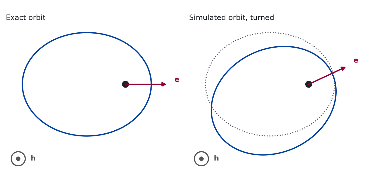
The two statements can be held in one picture. The conserved vectors are the angular momentum $\mathbf h$, which points out of the plane of the orbit and cannot turn, and the eccentricity vector $\mathbf e$, which points to the perihelion and is the one that a symplectic method lets turn:

def draw_orbit_conserved_vectors() -> Figure:
    """The eccentricity and angular momentum vectors of the exact and of a
    turned orbit, as a sketch."""
    fig, axes = plt.subplots(1, 2, figsize=(6.4, 3.2))
    eccentricity, semi_latus = 0.6, 1.0
    turn_simulated = np.radians(25.0)
    theta = np.linspace(0.0, 2.0 * np.pi, 300)
    radius = semi_latus / (1.0 + eccentricity * np.cos(theta))
    for ax, name, turn in zip(
        axes,
        ("Exact orbit", "Simulated orbit, turned"),
        (0.0, turn_simulated),
        strict=True,
    ):
        diagrams.frame(ax, (-2.9, 1.3), (-2.1, 1.9))
        ax.plot(
            radius * np.cos(theta),
            radius * np.sin(theta),
            color="#57606a",
            linestyle=":",
            linewidth=1.2,
        )
        ax.plot(
            radius * np.cos(theta + turn),
            radius * np.sin(theta + turn),
            color="#00429d",
            linewidth=1.6,
        )
        diagrams.circle(ax, (0.0, 0.0), 0.07, colour="#1f2328", filled=True)
        diagrams.arrow(
            ax, (0.0, 0.0), (1.0 * np.cos(turn), 1.0 * np.sin(turn)), colour=1
        )
        diagrams.text(
            ax,
            (1.1 * np.cos(turn) + 0.15, 1.1 * np.sin(turn) + 0.1),
            "$\\mathbf{e}$",
            colour=1,
        )
        diagrams.circle(ax, (-2.6, -1.8), 0.17, colour=2)
        diagrams.circle(ax, (-2.6, -1.8), 0.04, colour=2, filled=True)
        diagrams.text(ax, (-2.3, -1.8), "$\\mathbf{h}$", ha="left", colour=2)
        diagrams.text(ax, (-2.9, 1.6), name, ha="left")
    fig.tight_layout()
    return fig

src/pbc/mechanics/experiments/kepler_orbit.py, lines 74 to 117, read from the repository when this page was built.

Figure 1: conceptual The exact orbit, left, keeps the direction of the eccentricity vector e and the angular momentum h for ever. A symplectic method, right, keeps h and the size and shape of the ellipse, but turns e, so the whole ellipse turns a little with every orbit; the dotted ellipse is the exact one.

The sketch exaggerates the turn so that it can be seen; the size of the real one is measured in the worked example on precession. The picture says what the measurement is a measurement of: the angle between the two arrows $\mathbf e$, accumulated over the orbits, while $\mathbf h$ stays put.

The program

The reusable code lives in the module pbc.mechanics.orbit of the repository. It adds the gravitational force in both of its forms, the conserved quantities, the elements of the orbit, and the exact motion; the simulation itself, the integrators, the energies, and the system of several particles are those of the earlier lessons, imported from their modules. The listings in this section are read from the files when the site is built.

The force between two bodies, as a pairwise force for interacting, and the same force on one body about a fixed centre, as a force for newton:

def gravitational_attraction(G: float, m1: float, m2: float) -> PairwiseForce:
    """Newton's law of gravitation between two bodies of masses ``m1`` and
    ``m2``: the force -G m1 m2 r / |r|³ on the first, at the position r
    relative to the second, as a pairwise force for
    ``pbc.mechanics.particles.interacting``."""
    for name, value in (("G", G), ("m1", m1), ("m2", m2)):
        _check_positive(name, value)

    def force(r: Vector) -> Vector:
        return -G * m1 * m2 * r / np.sqrt(r @ r) ** 3

    return force

src/pbc/mechanics/orbit.py, lines 38 to 49, read from the repository when this page was built.

def central_gravity(gm: float, mass: float) -> Force:
    """The inverse-square force -GM m x / |x|³ on a body of ``mass`` at the
    position x from a fixed centre with the gravitational parameter ``gm``
    = G M. With ``mass`` the reduced mass and ``gm`` = G (m1 + m2) it is the
    force of the relative motion of two bodies."""
    _check_positive("gm", gm)
    _check_positive("mass", mass)

    def force(t: float, x: Vector, v: Vector) -> Vector:
        return -gm * mass * x / np.sqrt(x @ x) ** 3

    return force

src/pbc/mechanics/orbit.py, lines 52 to 63, read from the repository when this page was built.

def gravitational_potential(gm: float, mass: float) -> Potential:
    """The potential energy -GM m / |x| of ``central_gravity``, zero at
    infinite distance, so that a bound orbit has negative energy."""
    _check_positive("gm", gm)
    _check_positive("mass", mass)

    def potential(x: Vector) -> float:
        return float(-gm * mass / np.sqrt(x @ x))

    return potential

src/pbc/mechanics/orbit.py, lines 66 to 75, read from the repository when this page was built.

The angular momentum in the plane:

def angular_momentum(trajectory: Trajectory, mass: float) -> NDArray[np.float64]:
    """The angular momentum m (x v_y - y v_x) about the origin, in kg m²/s,
    at every instant of a ``trajectory`` in the plane: the component
    perpendicular to the plane, positive for anticlockwise motion. A central
    force keeps it constant."""
    _check_positive("mass", mass)
    return mass * _cross(trajectory.x, trajectory.v)

src/pbc/mechanics/orbit.py, lines 87 to 93, read from the repository when this page was built.

The elements of the orbit through a state, from the two conserved quantities, and the eccentricity vector:

@dataclass(frozen=True)
class Orbit:
    """The shape and the period of a bound orbit about a centre of
    attraction."""

    semi_major_axis: float  # a: half the longest diameter of the ellipse
    eccentricity: float  # e: 0 for a circle, approaching 1 for a long, thin ellipse
    period: float  # T = 2 pi sqrt(a³ / GM), Kepler's third law

    @property
    def periapsis(self) -> float:
        """The closest distance to the centre, a (1 - e)."""
        return self.semi_major_axis * (1.0 - self.eccentricity)

    @property
    def apoapsis(self) -> float:
        """The farthest distance from the centre, a (1 + e)."""
        return self.semi_major_axis * (1.0 + self.eccentricity)

src/pbc/mechanics/orbit.py, lines 96 to 113, read from the repository when this page was built.

def orbital_elements(state: State, gm: float) -> Orbit:
    """The orbit through ``state`` about a centre at the origin with the
    gravitational parameter ``gm``, from the two conserved quantities.

    With the energy per unit mass epsilon = |v|² / 2 - GM / |x| and the
    angular momentum per unit mass h = x v_y - y v_x,

        a = -GM / (2 epsilon),    e = sqrt(1 + 2 epsilon h² / GM²),
        T = 2 pi sqrt(a³ / GM).

    The eccentricity is evaluated as the length of ``eccentricity_vector``,
    which equals the square root above exactly but not in floating point:
    near a circle the expression under the root is the difference of two
    numbers close to 1, and its round-off of about 1e-16 becomes an
    eccentricity of about 1e-8 after the root, while the vector carries the
    round-off itself.

    The orbit must be bound, epsilon < 0; a state at or above the escape
    speed sqrt(2 GM / |x|) raises ``ValueError``. The orbit must also turn,
    h != 0: a body moving straight towards or away from the centre falls
    into it along a line, a degenerate ellipse of eccentricity 1 with no
    plane and no periapsis to orient it, and raises ``ValueError`` too.
    """
    _check_positive("gm", gm)
    r = np.sqrt(state.x @ state.x)
    epsilon = 0.5 * (state.v @ state.v) - gm / r
    if epsilon >= 0:
        raise ValueError(
            f"the orbit is not bound: the energy per unit mass is {epsilon:.4g},"
            " not negative"
        )
    if _cross(state.x, state.v) == 0.0:
        raise ValueError(
            "the orbit is radial: the angular momentum is zero, so the body"
            " falls into the centre along a line instead of tracing an ellipse"
        )
    a = -gm / (2.0 * epsilon)
    ecc = eccentricity_vector(state, gm)
    e = float(np.sqrt(ecc @ ecc))
    return Orbit(float(a), e, float(2.0 * np.pi * np.sqrt(a**3 / gm)))

src/pbc/mechanics/orbit.py, lines 116 to 155, read from the repository when this page was built.

def eccentricity_vector(state: State, gm: float) -> Vector:
    """The vector e = (|v|² x - (x . v) v) / GM - x / |x|, which points from
    the centre to the periapsis and has the eccentricity as its length. It
    is constant on the exact orbit; a simulation that turns it is
    precessing."""
    _check_positive("gm", gm)
    x, v = state.x, state.v
    return ((v @ v) * x - (x @ v) * v) / gm - x / np.sqrt(x @ x)

src/pbc/mechanics/orbit.py, lines 158 to 165, read from the repository when this page was built.

The exact motion, from Kepler’s equation:

def kepler_motion(initial: State, gm: float, t: ArrayLike) -> Trajectory:
    """The exact motion from ``initial`` about a centre at the origin with the
    gravitational parameter ``gm``, evaluated at the times ``t``.

    The orbit is the ellipse of ``orbital_elements``, oriented by the
    eccentricity vector. Each time is turned into the mean anomaly
    M = M_0 + n (t - t_0) with the mean motion n = 2 pi / T, Kepler's
    equation E - e sin E = M is solved for the eccentric anomaly E, and the
    position and velocity follow from E in the frame of the ellipse:

        x = a (cos E - e) P + a sqrt(1 - e²) sin E Q,
        v = sqrt(GM a) / |x| (-sin E P + sqrt(1 - e²) cos E Q),

    with P the unit vector towards the periapsis and Q the unit vector a
    quarter turn ahead in the direction of the motion. The orbit must be
    bound and must have a nonzero angular momentum, as for
    ``orbital_elements``; a radial infall raises ``ValueError``. ``t`` is a
    scalar or an array; the arrays of the result have one row per time.
    """
    orbit = orbital_elements(initial, gm)
    a, e = orbit.semi_major_axis, orbit.eccentricity
    n = 2.0 * np.pi / orbit.period
    h = float(_cross(initial.x, initial.v))
    ecc = eccentricity_vector(initial, gm)
    # e is the length of ecc, so P is a unit vector whenever e > 0, however
    # small. A circle has no periapsis; any direction then serves as the
    # reference, and the eccentric anomaly below is measured from it.
    P = ecc / e if e > 0.0 else initial.x / np.sqrt(initial.x @ initial.x)
    Q = np.sign(h) * np.array([-P[1], P[0]])
    b = a * np.sqrt(1.0 - e**2)
    # The eccentric anomaly at the initial time, from the position.
    E_0 = np.arctan2((initial.x @ Q) / b, (initial.x @ P) / a + e)
    M_0 = E_0 - e * np.sin(E_0)

    times = np.array(t, dtype=np.float64, ndmin=1)
    E = _solve_kepler(M_0 + n * (times - initial.t), e)
    cos, sin = np.cos(E)[:, np.newaxis], np.sin(E)[:, np.newaxis]
    x = a * (cos - e) * P + b * sin * Q
    r = a * (1.0 - e * np.cos(E))[:, np.newaxis]
    v = np.sqrt(gm * a) / r * (-sin * P + np.sqrt(1.0 - e**2) * cos * Q)
    return Trajectory(t=times, x=x, v=v)

src/pbc/mechanics/orbit.py, lines 179 to 219, read from the repository when this page was built.

The two steppers for which the angular momentum is conserved exactly, with the lines that carry the argument above marked. The order of the two updates is what makes it work:

def symplectic_euler_step(state: State, acceleration: Acceleration, dt: float) -> State:
    """Advance ``state`` by one symplectic Euler step of length ``dt`` (s).

    The velocity changes first, with the acceleration at the old state;
    then the *new* velocity moves the particle. One change of order against
    explicit Euler, with the same cost; it is the simplest method that keeps
    the energy of an oscillator bounded.
    """
    v = state.v + acceleration(state.t, state.x, state.v) * dt
    return State(t=state.t + dt, x=state.x + v * dt, v=v)

1. Line 24, v = state.v + acceleration(state.t, state.x, state.v) * dt: The velocity changes by a vector along the old position, so the cross product of the position with it is unchanged.
2. Line 25, return State(t=state.t + dt, x=state.x + v * dt, v=v): The position moves along the new velocity, which a cross product with the new velocity does not see. Moving it along the old velocity, as explicit Euler does, would.

src/pbc/mechanics/integrators.py, lines 16 to 25, read from the repository when this page was built.

def verlet_step(state: State, acceleration: Acceleration, dt: float) -> State:
    """Advance ``state`` by one velocity Verlet step of length ``dt`` (s).

    The position moves by the Taylor expansion to second order, with the
    acceleration at the old state; the velocity changes by the average of
    the old acceleration and the one at the new position. When the force
    depends on the velocity, the new acceleration is evaluated at the
    explicit Euler prediction of the new velocity, which keeps the method
    second order.
    """
    a = acceleration(state.t, state.x, state.v)
    t = state.t + dt
    x = state.x + state.v * dt + 0.5 * a * dt**2
    a_next = acceleration(t, x, state.v + a * dt)
    return State(t=t, x=x, v=state.v + 0.5 * (a + a_next) * dt)

1. Line 40, x = state.x + state.v * dt + 0.5 * a * dt**2: The position moves along the old velocity plus half a step of the old acceleration, the vector called w in the derivation.
2. Line 42, return State(t=t, x=x, v=state.v + 0.5 * (a + a_next) * dt): The part of the velocity change that comes from the new acceleration points along the new position and drops out of the cross product with it.

src/pbc/mechanics/integrators.py, lines 28 to 42, read from the repository when this page was built.

Worked examples

One orbit, four methods

The orbit of the examples has a semi-major axis of 1 AU and an eccentricity of 0.5 about a body of one solar mass. The orbiting body has the mass of the Earth, three millionths of a solar mass, which affects nothing but the units of the energy. The cell sets it up at the perihelion, takes the elements of the orbit from the state, and runs two orbits with each method at 100 steps per orbit against the exact motion. The table lists the largest distance from the exact position, the relative energy drift of the energy lesson, and the relative spread of the angular momentum.

gm = 4 * np.pi**2  # G times one solar mass, in AU³/yr²
planet_mass = 3.0e-6  # solar masses: the Earth
gravity = newton(planet_mass, central_gravity(gm, planet_mass))
potential = gravitational_potential(gm, planet_mass)
FLOOR = 1e-12  # below this, a conserved quantity is shown as a bound

src/pbc/mechanics/experiments/kepler_orbit.py, lines 44 to 48, read from the repository when this page was built.

def at_perihelion(a, e):
    """At the closest point of the orbit with these elements, moving
    anticlockwise."""
    r = a * (1 - e)
    return State(t=0.0, x=[r, 0.0], v=[0.0, np.sqrt(gm * (1 + e) / r)])

src/pbc/mechanics/experiments/kepler_orbit.py, lines 52 to 56, read from the repository when this page was built.

start = at_perihelion(1.0, 0.5)
ellipse = orbital_elements(start, gm)
metres_per_second = au / Julian_year  # one AU per year
perihelion_speed = np.linalg.norm(start.v) * metres_per_second / 1e3  # km/s

src/pbc/mechanics/experiments/kepler_orbit.py, lines 60 to 63, read from the repository when this page was built.

def shown(spread):
    """A spread at the level of round-off is shown as a bound, not as a number."""
    return f"{spread:.1e}" if spread > FLOOR else "below 1e-12"

src/pbc/mechanics/experiments/kepler_orbit.py, lines 120 to 122, read from the repository when this page was built.

def run_orbits(integrator, steps_per_orbit, n_orbits, initial=start):
    return simulate(
        initial,
        gravity,
        ellipse.period / steps_per_orbit,
        round(n_orbits * steps_per_orbit),
        step=integrator.step,
    )

src/pbc/mechanics/experiments/kepler_orbit.py, lines 125 to 132, read from the repository when this page was built.

def position_error(trajectory, initial=start):
    """The largest distance from the exact position over the run, in AU."""
    exact = kepler_motion(initial, gm, trajectory.t)
    return np.max(np.hypot(*(trajectory.x - exact.x).T))

src/pbc/mechanics/experiments/kepler_orbit.py, lines 135 to 138, read from the repository when this page was built.

def four_methods_two_orbits(experiment: Experiment) -> None:
    """Two orbits at one hundred steps per orbit with each method; record the
    table."""
    rows = []
    for integrator in INTEGRATORS:
        trajectory = run_orbits(integrator, 100, 2)
        energies = mechanical_energy(trajectory, planet_mass, potential)
        momenta = angular_momentum(trajectory, planet_mass)
        rows.append(
            (
                integrator.name,
                position_error(trajectory),
                energy_drift(energies),
                shown(np.ptp(momenta) / momenta[0]),
            )
        )

    experiment.table(
        "four-methods-two-orbits",
        rows,
        columns=[
            ("method", "", ""),
            ("largest position error", "AU", ".1e"),
            ("energy drift", "", ".1e"),
            ("angular momentum spread", "", ""),
        ],
        caption="Two orbits at one hundred steps per orbit: position error, "
        "relative energy drift, and relative spread of the angular momentum; a "
        "spread at round-off level is shown as a bound.",
    )

src/pbc/mechanics/experiments/kepler_orbit.py, lines 141 to 170, read from the repository when this page was built.

Two orbits at one hundred steps per orbit: position error, relative energy drift, and relative spread of the angular momentum; a spread at round-off level is shown as a bound.

method	largest position error (AU)	energy drift	angular momentum spread
explicit Euler	6.4e+00	7.4e-01	2.8e-01
symplectic Euler	7.8e-01	1.2e-01	below 1e-12
velocity Verlet	3.5e-01	1.1e-02	below 1e-12
Runge-Kutta 4	1.6e-03	6.3e-05	9.2e-06

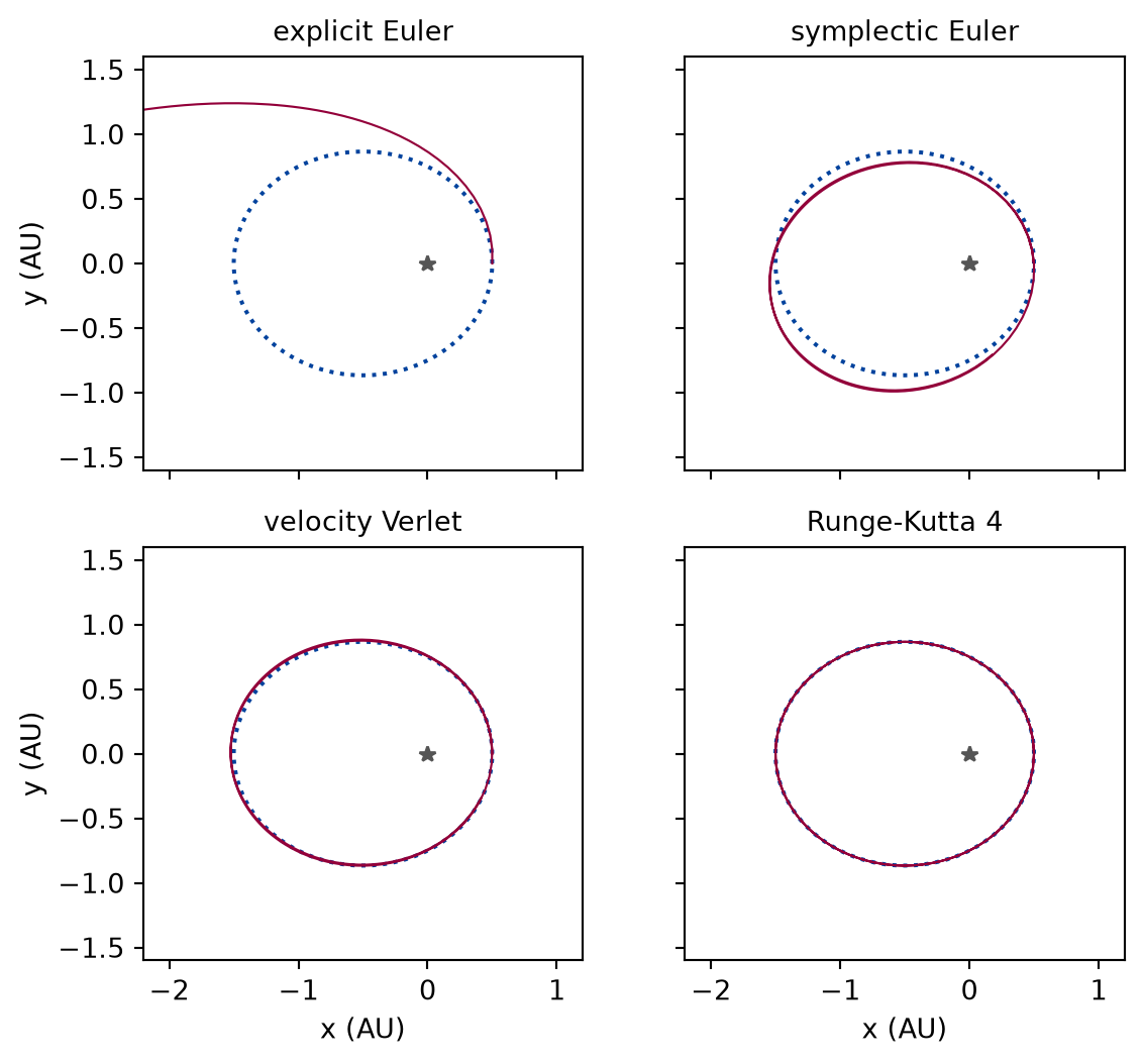
The elements the state gives are a semi-major axis of 1.0000 AU, an eccentricity of 0.5000, and a period of 1.0000 yr, with the perihelion at 0.50 AU, where the planet moves at 51.6 km/s, and the aphelion at 1.50 AU. Numerically verified (the example orbit at this step): The two symplectic methods conserve the angular momentum to round-off at a step of a hundredth of an orbit, while explicit Euler and the classical Runge-Kutta method do not. This is the new result, as the derivation says. The energy behaves as on the oscillator and the pendulum, and the position error after two orbits ranks the methods by their order, as before: the classical Runge-Kutta method is the method for an accurate position over a short run.

def draw_orbit_four_methods() -> Figure:
    """Two orbits of each method against the exact ellipse."""
    exact_orbit = kepler_motion(start, gm, np.linspace(0.0, ellipse.period, 400))

    fig, axes = plt.subplots(2, 2, figsize=(6.4, 5.6), sharex=True, sharey=True)
    for ax, integrator in zip(axes.flat, INTEGRATORS, strict=True):
        trajectory = run_orbits(integrator, 100, 2)
        ax.plot(
            exact_orbit.x[:, 0],
            exact_orbit.x[:, 1],
            color="#00429d",
            linestyle=":",
            label="exact",
        )
        ax.plot(trajectory.x[:, 0], trajectory.x[:, 1], color="#93003a", linewidth=0.8)
        ax.plot(0, 0, color="#555555", marker="*", linestyle="none")
        ax.set_title(integrator.name, fontsize=10)
        ax.set_xlim(-2.2, 1.2)
        ax.set_ylim(-1.6, 1.6)
        ax.set_aspect("equal")
    for ax in axes[1]:
        ax.set_xlabel("x (AU)")
    for ax in axes[:, 0]:
        ax.set_ylabel("y (AU)")
    fig.tight_layout()
    return fig

src/pbc/mechanics/experiments/kepler_orbit.py, lines 173 to 198, read from the repository when this page was built.

Figure 2: simulated Two orbits with each method at the same step, against the exact ellipse, with the star at the origin. Explicit Euler spirals out of the picture; the two symplectic methods stay on ellipses of about the right size that are turned against the exact one; the classical Runge-Kutta method cannot be told from it.

The figure draws the runs of the table against the exact motion of kepler_motion; the turned ellipses of the two symplectic methods are the precession that the next example measures. The next cell confirms the orders by halving the step.

step_counts = [200, 400, 800, 1600, 3200]

src/pbc/mechanics/experiments/kepler_orbit.py, line 67, read from the repository when this page was built.

def observed_orders(experiment: Experiment) -> dict:
    """The largest position error over two orbits for each method and step
    count, with the observed order; record the table and return the
    errors."""
    errors = {
        integrator.name: np.array(
            [position_error(run_orbits(integrator, n, 2)) for n in step_counts]
        )
        for integrator in INTEGRATORS
    }

    columns = [("steps per orbit", "", "d")]
    for integrator in INTEGRATORS:
        columns += [
            (f"{integrator.name}: error", "AU", ".1e"),
            (f"{integrator.name}: order", "", ".2f"),
        ]
    rows = []
    for i, n in enumerate(step_counts):
        row = [n]
        for integrator in INTEGRATORS:
            error = errors[integrator.name]
            row += [error[i], np.log2(error[i - 1] / error[i]) if i else None]
        rows.append(row)

    experiment.table(
        "observed-orders",
        rows,
        columns=columns,
        caption="Largest position error over two orbits for each method, and the "
        "observed order from the previous row, to two decimals.",
    )
    return errors

src/pbc/mechanics/experiments/kepler_orbit.py, lines 201 to 233, read from the repository when this page was built.

Largest position error over two orbits for each method, and the observed order from the previous row, to two decimals.

steps per orbit	explicit Euler: error (AU)	explicit Euler: order	symplectic Euler: error (AU)	symplectic Euler: order	velocity Verlet: error (AU)	velocity Verlet: order	Runge-Kutta 4: error (AU)	Runge-Kutta 4: order
200	3.2e+00		2.2e-01		8.9e-02		6.7e-05
400	2.9e+00	0.18	6.8e-02	1.68	2.2e-02	2.00	3.2e-06	4.38
800	2.7e+00	0.09	3.5e-02	0.95	5.5e-03	2.00	1.7e-07	4.23
1600	2.0e+00	0.41	1.8e-02	0.97	1.4e-03	2.00	9.8e-09	4.13
3200	1.4e+00	0.58	9.0e-03	0.99	3.5e-04	2.00	5.9e-10	4.07

Numerically verified (the example orbit, two orbits): Velocity Verlet shows its second order at once, and the classical Runge-Kutta method approaches its fourth from above as the step becomes small enough for the fast perihelion passage. The first-order methods take longer to settle. Explicit Euler is nowhere near its asymptotic regime at these steps: at the finest step its error is still 1.4 times the semi-major axis, because the energy it feeds in during each perihelion passage changes the orbit itself, so the error is no longer a small perturbation of the exact orbit. The accuracy question has the same answer as on the oscillator. The long-run question does not.

A thousand orbits

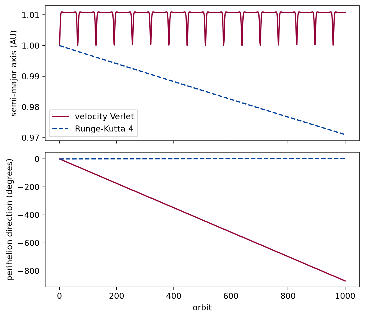
The cell runs a thousand orbits with velocity Verlet and with the classical Runge-Kutta method at a hundred steps per orbit. At the end of every orbit it asks which ellipse the body is on: the semi-major axis from the energy and the direction of the perihelion from the eccentricity vector.

n_orbits, steps_per_orbit = 1000, 100

src/pbc/mechanics/experiments/kepler_orbit.py, line 70, read from the repository when this page was built.

def once_per_orbit(trajectory):
    """The state at the end of every orbit."""
    return [
        State(trajectory.t[i], trajectory.x[i], trajectory.v[i])
        for i in range(0, len(trajectory.t), steps_per_orbit)
    ]

src/pbc/mechanics/experiments/kepler_orbit.py, lines 236 to 241, read from the repository when this page was built.

def perihelion_direction(states):
    """The angle of the eccentricity vector, in degrees, unwrapped."""
    vectors = np.array([eccentricity_vector(state, gm) for state in states])
    return np.degrees(np.unwrap(np.arctan2(vectors[:, 1], vectors[:, 0])))

src/pbc/mechanics/experiments/kepler_orbit.py, lines 244 to 247, read from the repository when this page was built.

def thousand_orbits(experiment: Experiment):
    """A thousand orbits with velocity Verlet and Runge-Kutta 4; record the
    table and return the runs and their statistics."""
    long_runs = {
        integrator.name: run_orbits(integrator, steps_per_orbit, n_orbits)
        for integrator in (verlet, rk4)
    }

    long_stats = {}
    rows = []
    for integrator in (verlet, rk4):
        trajectory = long_runs[integrator.name]
        energies = mechanical_energy(trajectory, planet_mass, potential)
        momenta = angular_momentum(trajectory, planet_mass)
        axes_over_time = np.array(
            [
                orbital_elements(state, gm).semi_major_axis
                for state in once_per_orbit(trajectory)
            ]
        )
        turned = perihelion_direction(once_per_orbit(trajectory))
        long_stats[integrator.name] = {
            "axis_min": axes_over_time.min(),
            "axis_max": axes_over_time.max(),
            "turned": turned[-1] - turned[0],
        }
        rows.append(
            (
                integrator.name,
                energy_drift(energies[: 100 * steps_per_orbit + 1]),
                energy_drift(energies),
                shown(np.ptp(momenta) / momenta[0]),
                axes_over_time.min(),
                axes_over_time.max(),
                turned[-1] - turned[0],
                (turned[-1] - turned[0]) / n_orbits,
            )
        )

    experiment.table(
        "thousand-orbits",
        rows,
        columns=[
            ("method", "", ""),
            ("energy drift, first hundred orbits", "", ".1e"),
            ("energy drift, all orbits", "", ".1e"),
            ("angular momentum spread", "", ""),
            ("smallest semi-major axis", "AU", ".4f"),
            ("largest semi-major axis", "AU", ".4f"),
            ("perihelion turned in all", "degrees", "+.1f"),
            ("perihelion turned per orbit", "degrees", "+.3f"),
        ],
        caption="A thousand orbits at a hundred steps per orbit: energy drift over "
        "the first hundred and over all orbits, spread of the angular momentum, "
        "range of the semi-major axis at the end of each orbit, and the turn of "
        "the perihelion.",
    )
    return long_runs, long_stats

src/pbc/mechanics/experiments/kepler_orbit.py, lines 250 to 307, read from the repository when this page was built.

A thousand orbits at a hundred steps per orbit: energy drift over the first hundred and over all orbits, spread of the angular momentum, range of the semi-major axis at the end of each orbit, and the turn of the perihelion.

method	energy drift, first hundred orbits	energy drift, all orbits	angular momentum spread	smallest semi-major axis (AU)	largest semi-major axis (AU)	perihelion turned in all (degrees)	perihelion turned per orbit (degrees)
velocity Verlet	1.1e-02	1.1e-02	below 1e-12	1.0000	1.0110	-872.3	-0.872
Runge-Kutta 4	3.0e-03	3.0e-02	4.7e-03	0.9710	1.0000	+4.6	+0.005

def draw_orbit_thousand(long_runs: dict) -> Figure:
    """The semi-major axis and the perihelion direction over a thousand
    orbits."""
    fig, (top, bottom) = plt.subplots(2, 1, figsize=(6.4, 5.6), sharex=True)
    for integrator, style in ((verlet, "-"), (rk4, "--")):
        states = once_per_orbit(long_runs[integrator.name])
        orbit_number = np.arange(len(states))
        top.plot(
            orbit_number,
            [orbital_elements(state, gm).semi_major_axis for state in states],
            color="#93003a" if integrator is verlet else "#00429d",
            linestyle=style,
            label=integrator.name,
        )
        bottom.plot(
            orbit_number,
            perihelion_direction(states),
            color="#93003a" if integrator is verlet else "#00429d",
            linestyle=style,
            label=integrator.name,
        )
    top.set_ylabel("semi-major axis (AU)")
    top.legend(loc="lower left")
    bottom.set_xlabel("orbit")
    bottom.set_ylabel("perihelion direction (degrees)")
    fig.tight_layout()
    return fig

src/pbc/mechanics/experiments/kepler_orbit.py, lines 310 to 336, read from the repository when this page was built.

Figure 3: simulated The semi-major axis of the ellipse the body is on, and the direction of its perihelion, at the end of every orbit. Velocity Verlet keeps the size of the ellipse and turns it at a steady rate; the classical Runge-Kutta method holds the direction and shrinks the ellipse at a steady rate.

The two methods fail in opposite ways. Numerically verified (the example orbit at this step): Velocity Verlet’s energy band is as wide after a thousand orbits as after one, its angular momentum is exact to round-off, and the semi-major axis stays within 1.1 per cent of the truth for the whole run. What it gets wrong is the direction of the ellipse, which turns at a steady rate and has gone round 2.4 times. Numerically verified (the example orbit at this step): The classical Runge-Kutta method holds the direction but loses energy at every step, so its ellipse shrinks by 2.9 per cent in a thousand orbits, and with it the period. That orbit is a different orbit by then. The energy of the symplectic method is trustworthy; its position after a thousand orbits is not, and the precession is the measure of how much it is not. The cell measures it against the step.

def precession_against_step(experiment: Experiment) -> None:
    """The precession of the perihelion per orbit for velocity Verlet at
    three steps; record the table."""
    rows, previous = [], None
    for n in (100, 200, 400):
        final = run_orbits(verlet, n, 50)
        turned = (
            perihelion_direction([State(final.t[-1], final.x[-1], final.v[-1])])[0] / 50
        )
        rows.append((n, turned, turned / previous if previous else None))
        previous = turned

    experiment.table(
        "precession-against-step",
        rows,
        columns=[
            ("steps per orbit", "", "d"),
            ("perihelion turned per orbit", "degrees", "+.4f"),
            ("ratio to the row above", "", ".3f"),
        ],
        caption="Precession of the perihelion per orbit for velocity Verlet over "
        "fifty orbits, for three steps, and its ratio to the coarser step.",
    )

src/pbc/mechanics/experiments/kepler_orbit.py, lines 339 to 361, read from the repository when this page was built.

Precession of the perihelion per orbit for velocity Verlet over fifty orbits, for three steps, and its ratio to the coarser step.

steps per orbit	perihelion turned per orbit (degrees)	ratio to the row above
100	-0.8775
200	-0.2208	0.252
400	-0.0550	0.249

Numerically verified (velocity Verlet, the example orbit): The precession falls by a factor of four when the step halves. It is a second-order error, like everything else about the method, and a run that needs the perihelion to stay put to a given angle over a given number of orbits chooses its step from this table. The position error of a symplectic method grows linearly in time, as the phase lag of the pendulum did, with the energy in its band all the while. The figure and the tables are one run of one orbit; the precession rate for other eccentricities was not measured.

Two bodies

The reduction to one body is an exact identity of the equations. The cell checks that the simulation respects it: a star of one solar mass and a planet of one thousandth, about the mass of Jupiter, on the same orbit, simulated as two interacting particles with the code of the momentum lesson, against the one-body simulation with the reduced mass and $G(m_1 + m_2)$. The centre of mass starts at rest at the origin.

def two_body_simulation(experiment: Experiment):
    """A heavy planet and its star as two bodies over five orbits, against
    the one-body run of their relative motion; record the table and return
    the positions and the speeds of the star, in m/s."""
    star_mass, heavy_planet = 1.0, 1.0e-3  # solar masses
    total_mass = star_mass + heavy_planet
    mu = reduced_mass(star_mass, heavy_planet)
    two_bodies = interacting(
        [star_mass, heavy_planet],
        gravitational_attraction(gm, star_mass, heavy_planet),
    )

    relative = State(
        t=0.0, x=[0.5, 0.0], v=[0.0, np.sqrt(gm * total_mass * 1.5 / 0.5)]
    )  # e = 0.5 again
    both = State(
        t=0.0,
        x=stack(
            [
                -heavy_planet / total_mass * relative.x,
                star_mass / total_mass * relative.x,
            ]
        ),
        v=stack(
            [
                -heavy_planet / total_mass * relative.v,
                star_mass / total_mass * relative.v,
            ]
        ),
    )
    pair_orbit = orbital_elements(relative, gm * total_mass)
    dt = pair_orbit.period / 200
    as_two = simulate(both, two_bodies, dt, 5 * 200, step=verlet.step)
    as_one = simulate(
        relative,
        newton(mu, central_gravity(gm * total_mass, mu)),
        dt,
        5 * 200,
        step=verlet.step,
    )

    positions, velocities = unstack(as_two.x, 2), unstack(as_two.v, 2)
    star_speed = np.linalg.norm(velocities[:, 0], axis=1) * metres_per_second
    centre_drift = np.max(np.abs(centre_of_mass([star_mass, heavy_planet], positions)))
    difference = np.max(np.abs((positions[:, 1] - positions[:, 0]) - as_one.x))
    bound = 1e-9  # AU, far above round-off and far below any other length

    experiment.table(
        "two-body-simulation",
        [
            ("period of the pair", "yr", f"{pair_orbit.period:.5f}"),
            (
                "drift of the centre of mass below the bound",
                "",
                "yes" if centre_drift < bound else "no",
            ),
            (
                "difference from the one-body run below the bound",
                "",
                "yes" if difference < bound else "no",
            ),
            ("slowest speed of the star", "m/s", f"{star_speed.min():.1f}"),
            ("fastest speed of the star", "m/s", f"{star_speed.max():.1f}"),
        ],
        columns=[("quantity", "", ""), ("unit", "", ""), ("value", "", "")],
        caption="The two bodies as two bodies over five orbits: the period, "
        "whether the centre of mass and the relative position agree with the "
        "one-body statements to a bound of 1e-9 AU, and the speed of the star.",
    )
    return positions, star_speed

src/pbc/mechanics/experiments/kepler_orbit.py, lines 364 to 433, read from the repository when this page was built.

The two bodies as two bodies over five orbits: the period, whether the centre of mass and the relative position agree with the one-body statements to a bound of 1e-9 AU, and the speed of the star.

quantity	unit	value
period of the pair	yr	0.99950
drift of the centre of mass below the bound		yes
difference from the one-body run below the bound		yes
slowest speed of the star	m/s	17.1
fastest speed of the star	m/s	51.6

def draw_two_bodies(positions) -> Figure:
    """The paths of the planet and of the star about the centre of mass."""
    fig, ax = plt.subplots(figsize=(6.4, 4.2))
    ax.plot(positions[:, 1, 0], positions[:, 1, 1], color="#93003a", label="planet")
    ax.plot(
        1000 * positions[:, 0, 0],
        1000 * positions[:, 0, 1],
        color="#00429d",
        linestyle="--",
        label="star, ×1000",  # noqa: RUF001, the multiplication sign
    )
    ax.plot(0, 0, color="#555555", marker="+", linestyle="none", label="centre of mass")
    ax.set_aspect("equal")
    ax.set_xlabel("x (AU)")
    ax.set_ylabel("y (AU)")
    ax.legend(loc="upper left")
    return fig

src/pbc/mechanics/experiments/kepler_orbit.py, lines 436 to 452, read from the repository when this page was built.

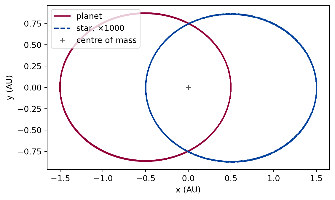
Figure 4: simulated The two bodies about their common centre of mass over five orbits: the planet’s ellipse and, magnified a thousandfold, the star’s, which has the same shape on the opposite side.

Numerically verified (velocity Verlet, five orbits): The two simulations agree, as they must: the same method and the same step applied to the same equations in two forms. The star moves on an ellipse a thousand times smaller than the planet’s, opposite to it, at between 17 and 52 metres per second. That motion is visible in the star’s light, as a periodic Doppler shift, and it is how planets around other stars are found. Observational (the radial velocity method): The first planet confirmed around a star like the Sun was found this way. The third exercise computes the speed for Jupiter and the Sun.

Go deeper: Doppler spectroscopy (Wikipedia, introduction and History (first paragraphs), and the Jupiter and Sun example; intuition.)

How the wobble of a star becomes a measurement: the Doppler shift of its spectrum, the instruments that reached the size of the effect, and what the amplitude gives for the mass of the planet. The lesson does not need it; it shows only the motion that the method measures.

Limits

What this lesson shows is a statement about one force law and four fixed-step methods on one orbit, not about orbital mechanics in general.

• The exact motion and the formulas for $a$, $e$, and $T$ are specific to the two-body problem. Generic three-body motion follows no fixed Keplerian ellipse and has no general closed form, so $a$, $e$, and $T$ describe the instant and not the future, and there is no exact motion to measure against. (Some special three-body solutions are periodic.)
• The long-run results are for one eccentricity and one step. That the precession falls with the square of the step is measured at three steps; that it grows with the eccentricity, or that a method with a variable step would behave differently, is not measured here.
• The elements come from the energy and the angular momentum as the code evaluates them in floating point. They are exact for the exact state and show the state of the simulation, not its error: the position error comes only from the comparison with kepler_motion.
• The precession shown is an error of the method. The real orbits of the planets precess for other reasons (the other planets, general relativity), which this lesson does not model and does not claim to separate from it.
• Nothing proved here is a theorem in Lean; the derivations are on the page and the checks are numerical.
• The wobble is the speed of the star about the centre of mass for an orbit seen from above. A real measurement gets only the component along the line of sight, and the inclination of the orbit hides part of the amplitude.

Self-check. Velocity Verlet conserves the angular momentum of the orbit exactly at every step, and its energy stays in a band. Does it follow that the simulated planet stays on the exact ellipse for a thousand orbits? Say what the long-run table shows, and which of the three constants is the one that fails.

With scripts, you can record in this browser that you answered this question.

Solution to the self-check

No. The angular momentum and the energy fix the size and the shape of the ellipse ($a$ and $e$), and they do not fix its direction. The eccentricity vector is the third constant, and the method does not conserve it: in the long run its direction has turned by 872 degrees, with the angular momentum at round-off and the semi-major axis within 1.1 per cent of the start. A planet on an ellipse of the right size and shape but turned by that angle is at the wrong place at the wrong time, although every conserved quantity that the earlier lessons monitor says the run is healthy. The first assumption that fails is the one about what “accurate” means: bounded energy and exact angular momentum say that the state lies on a slightly wrong ellipse, not that it lies where the exact motion is.

Exercises

Exercise 1. Kepler’s third law. Put a body on circular orbits with radii of 0.5, 1, 2, and 4 AU, simulate each with the classical Runge-Kutta method at 200 steps per orbit, and measure the period as the time between two crossings of the $x$ axis in the same direction. Check $T^2 / a^3$.

Solution to exercise 1

On a circular orbit the speed is $\sqrt{GM/a}$. The crossing times are interpolated within the step, as the period of the pendulum was.

def third_law(experiment: Experiment) -> list:
    """Exercise 1: the period of circular orbits at four radii, measured from
    the crossings of the x axis; record the table and return its rows."""
    third_law_rows = []
    for a in (0.5, 1.0, 2.0, 4.0):
        circular = State(t=0.0, x=[a, 0.0], v=[0.0, np.sqrt(gm / a)])
        period = 2 * np.pi * np.sqrt(a**3 / gm)
        trajectory = simulate(
            circular, gravity, period / 200, 2 * 200 + 10, step=rk4.step
        )
        y = trajectory.x[:, 1]
        before = np.where((y[:-1] < 0) & (y[1:] >= 0))[0]
        crossing = trajectory.t[before] - y[before] / (y[before + 1] - y[before]) * (
            trajectory.t[before + 1] - trajectory.t[before]
        )
        third_law_rows.append((a, crossing[0], crossing[0] ** 2 / a**3))

    experiment.table(
        "third-law",
        third_law_rows,
        columns=[
            ("radius", "AU", ".1f"),
            ("measured period", "yr", ".4f"),
            ("T² / a³", "yr² / AU³", ".4f"),
        ],
        caption="Period of a circular orbit measured from the crossings of the x "
        "axis, and T² / a³, to four decimals.",
    )
    return third_law_rows

src/pbc/mechanics/experiments/kepler_orbit.py, lines 455 to 483, read from the repository when this page was built.

Period of a circular orbit measured from the crossings of the x axis, and T² / a³, to four decimals.

radius (AU)	measured period (yr)	T² / a³ (yr² / AU³)
0.5	0.3536	1.0000
1.0	1.0000	1.0000
2.0	2.8284	1.0000
4.0	8.0000	1.0000

The ratio is the same for every radius, equal to 1.0000 $\mathrm{yr}^2/\mathrm{AU}^3$ to the precision of the table, which is the content of the law and the reason for the units: it depends on the mass of the central body and on nothing else about the orbit.

Exercise 2. Escape. At the perihelion of the example orbit, 0.5 AU from the star, the escape speed is $\sqrt{2GM/r}$. Launch a body from there at 99 per cent and at 101 per cent of it, simulate thirty years with the classical Runge-Kutta method, and ask orbital_elements about each.

Solution to exercise 2

Just below the escape speed the energy is slightly negative: a long, thin ellipse that comes back. Just above it the energy is positive and there is no ellipse to report.

launch_distance = 0.5  # AU
escape_speed = np.sqrt(2 * gm / launch_distance)

src/pbc/mechanics/experiments/kepler_orbit.py, lines 487 to 488, read from the repository when this page was built.

def escape(experiment: Experiment) -> list:
    """Exercise 2: launches at 99 and 101 per cent of the escape speed;
    record the table and return its rows."""
    escape_rows = []
    for fraction in (0.99, 1.01):
        launched = State(
            t=0.0, x=[launch_distance, 0.0], v=[0.0, fraction * escape_speed]
        )
        trajectory = simulate(launched, gravity, 0.005, 6000, step=rk4.step)
        distance = np.hypot(*trajectory.x.T)
        try:
            elements = orbital_elements(launched, gm)
            axis, ecc, period_text = (
                elements.semi_major_axis,
                elements.eccentricity,
                f"{elements.period:.0f}",
            )
        except ValueError:
            axis, ecc, period_text = None, None, "not bound"
        escape_rows.append(
            (100 * fraction, distance[-1], distance.max(), axis, ecc, period_text)
        )

    experiment.table(
        "escape",
        escape_rows,
        columns=[
            ("launch speed", "per cent of escape", ".0f"),
            ("distance after thirty years", "AU", ".1f"),
            ("farthest distance", "AU", ".1f"),
            ("semi-major axis", "AU", ".1f"),
            ("eccentricity", "", ".3f"),
            ("period", "yr", ""),
        ],
        caption="Two launches from the perihelion of the example orbit, at 99 and "
        "at 101 per cent of the escape speed, and what orbital_elements reports.",
    )
    return escape_rows

src/pbc/mechanics/experiments/kepler_orbit.py, lines 492 to 529, read from the repository when this page was built.

Two launches from the perihelion of the example orbit, at 99 and at 101 per cent of the escape speed, and what orbital_elements reports.

launch speed (per cent of escape)	distance after thirty years (AU)	farthest distance (AU)	semi-major axis (AU)	eccentricity	period (yr)
99	22.7	24.6	12.6	0.960	45
101	74.2	74.2			not bound

The escape speed at that distance is 12.566 AU/yr, or 59.6 km/s. A small difference in the launch speed is the difference between a comet that returns in 45 years and one that never does, and the energy knows it at the moment of launch. The simulation of the bound case needs the whole orbit to confirm what the two conserved quantities said from the first state.

Exercise 3. The wobble of the Sun. Jupiter has a mass of 0.000955 solar masses, a semi-major axis of 5.20 AU, and an eccentricity of 0.049. Simulate the Sun and Jupiter as two bodies for one orbit and print the speed of the Sun about the common centre of mass, in metres per second. Compare with the estimate for a circular orbit, the planet’s speed times $m_2 / M$.

Solution to exercise 3

def sun_and_jupiter(experiment: Experiment):
    """Exercise 3: the Sun and Jupiter as two bodies over one orbit; record
    the table and return the period, in yr, the speeds of the Sun, and the
    circular estimate, in m/s."""
    jupiter_mass, jupiter_a, jupiter_e = 0.000955, 5.20, 0.049
    total = 1.0 + jupiter_mass
    pair = interacting(
        [1.0, jupiter_mass], gravitational_attraction(gm, 1.0, jupiter_mass)
    )

    jupiter_r = jupiter_a * (1 - jupiter_e)
    jupiter_relative = State(
        t=0.0,
        x=[jupiter_r, 0.0],
        v=[0.0, np.sqrt(gm * total * (1 + jupiter_e) / jupiter_r)],
    )
    jupiter_both = State(
        t=0.0,
        x=stack(
            [
                -jupiter_mass / total * jupiter_relative.x,
                1.0 / total * jupiter_relative.x,
            ]
        ),
        v=stack(
            [
                -jupiter_mass / total * jupiter_relative.v,
                1.0 / total * jupiter_relative.v,
            ]
        ),
    )
    jupiter_period = orbital_elements(jupiter_relative, gm * total).period
    jupiter_run = simulate(
        jupiter_both, pair, jupiter_period / 400, 400, step=verlet.step
    )
    sun_speed = (
        np.linalg.norm(unstack(jupiter_run.v, 2)[:, 0], axis=1) * metres_per_second
    )
    circular_estimate = (
        jupiter_mass / total * np.sqrt(gm * total / jupiter_a) * metres_per_second
    )

    experiment.table(
        "sun-and-jupiter",
        [
            ("slowest speed of the Sun", sun_speed.min()),
            ("fastest speed of the Sun", sun_speed.max()),
            ("circular estimate", circular_estimate),
        ],
        columns=[("quantity", "", ""), ("speed", "m/s", ".1f")],
        caption="The speed of the Sun about the centre of mass of the Sun and "
        "Jupiter over one orbit, from the two-body simulation, and the circular "
        "estimate, to one decimal.",
    )
    return jupiter_period, sun_speed, circular_estimate

src/pbc/mechanics/experiments/kepler_orbit.py, lines 532 to 586, read from the repository when this page was built.

The speed of the Sun about the centre of mass of the Sun and Jupiter over one orbit, from the two-body simulation, and the circular estimate, to one decimal.

quantity	speed (m/s)
slowest speed of the Sun	11.9
fastest speed of the Sun	13.1
circular estimate	12.5

The period of Jupiter comes out as 11.85 yr. The Sun moves at between 11.9 and 13.1 m/s about the centre of mass, and the circular estimate is 12.5 m/s: about a dozen metres per second, a brisk cycling speed, over 12 years. Observational (the Sun and Jupiter, as quoted): The overview of the radial velocity method quotes the same effect for Jupiter and the Sun: about 12.4 m/s (not verified), as the change of the speed of the Sun over one orbit of Jupiter. The simulated range and the circular estimate bracket it. Detecting it in the spectrum of a star across light years is the radial velocity method of exoplanet astronomy, and the two-body code of this page is its model.

Run this experiment

This page was built from commit 6417e2ff90258bd2d2ba21d217eb7666fd24f680 of the repository.

In a clone at that commit, with the project’s Python packages installed, this command runs the experiment of this page:

uv run --locked --no-dev python -m pbc.mechanics.experiments.kepler_orbit results

Files, tests, and every command

The files behind it:

• site/lessons/mechanics/08-kepler-orbit/index.qmd: this page, with every code cell.
• src/pbc/mechanics/dynamics.py: code the experiment runs.
• src/pbc/mechanics/integrators.py: code the experiment runs.
• src/pbc/mechanics/energy.py: code the experiment runs.
• src/pbc/mechanics/particles.py: code the experiment runs.
• src/pbc/mechanics/orbit.py: code the experiment runs.
• src/pbc/mechanics/experiments/kepler_orbit.py: code the experiment runs.
• src/pbc/experiment.py: code the experiment runs.
• tests/unit/test_dynamics.py: tests of that code.
• tests/unit/test_integrators.py: tests of that code.
• tests/unit/test_energy.py: tests of that code.
• tests/unit/test_particles.py: tests of that code.
• tests/unit/test_orbit.py: tests of that code.
• tests/unit/test_kepler_orbit_experiment.py: tests of that code.

With Git and uv installed (see the setup page), run:

git clone https://github.com/taspinar/physics-by-construction.git
cd physics-by-construction
git checkout 6417e2ff90258bd2d2ba21d217eb7666fd24f680
uv sync --locked --no-dev
uv run --locked --no-dev python -m pbc.mechanics.experiments.kepler_orbit results

The experiment writes every figure of this page into results/, as <label>.png, and every number and table of the page, as the page shows it, into results/results.json. Its numbers match this page to the digits shown, and its figure files are the ones the page shows; digits beyond those can differ between machines, because floating-point libraries differ. Change the code of the experiment and run it again to see what changes.