Inverse physics: parameters from observations

Fitting a model to observations to find its parameters: how to check a fit against known answers, how to state the uncertainty, how to see that the data cannot tell two parameters apart or that the model is wrong, and what that means for the chirp mass read from the gravitational-wave strain.

Course

Classical mechanics, lesson 21 of 28

Slot

D6, number 6 of the 13 slots of the path Scientific law discovery

Methods

Simulation, Measured data

Difficulty

Advanced, level 3 of 3

What you’ll learn

Check a fitting procedure on synthetic data of known parameters, and say what recovery, bias, and coverage of the stated interval mean
Tell from a profile of the chi-square whether the data bound a parameter, and recognise two parameters that appear only as a combination
List the reasons not to take a converged fit as evidence for its model
State the uncertainty of a parameter fitted to measured data, with the scatter that an injection of a known signal shows

Prerequisites

The harmonic oscillator, Gravitational-wave strain lab.

Before you begin

Statistics: least squares, the chi-square of residuals, and a standard error

Related

none

Previous

Gravitational-wave strain lab

Next

Double pendulum and chaos

With scripts, this page keeps a record in your browser of whether you completed the lesson. Nothing is stored without them.

With scripts, this place suggests what to do next, with the reason, from the progress saved in your browser. Without them, follow the learning path.

The earlier lessons went from parameters to motion: give the mass and the spring constant, get the trajectory. A laboratory goes the other way. It has the trajectory, noisy, and wants the mass and the spring constant. That is an inverse problem, and it is harder than it looks for a reason that no amount of computing removes: a fit always returns numbers. The optimiser converges whether or not the data determine them, whether or not the model is right, and whether or not the stated error is the real one.

The lesson builds the checks one at a time. First a fit is run on synthetic data whose parameters are known, so that the answer can be compared with the truth. Then two ways a fit can converge and mean nothing: parameters that only appear as a combination, and a model that is wrong. Last, the fit of the gravitational-wave lesson is put through the same questions on the measured strain, and the uncertainty it deserves is stated.

Assumptions

The model is a function of the parameters and of the independent variable alone. Everything the observation depends on besides the parameters is fixed in the model. A fit cannot tell a wrong parameter from a wrong fixed value.
The noise is independent, Gaussian, and of known standard deviation. The chi-square, the covariance, and the interval from the profile all rest on it. The residuals are the place to look when it fails, and the measured case below is one where it does.
The uncertainty is small enough for a straight-line picture. The standard errors from the covariance linearise the model at the best fit. The profile of the chi-square does not, and the lesson uses both to see where they differ.
One minimum. The optimiser starts near the truth in the synthetic cases. A real fit can end in another local minimum; the profile walks across the parameter to see this.
A fit is a statement about a model. It says which parameters make the model closest to the data. It does not say that the model is the right one.

From a trajectory to its parameters

A fit is checked against a known answer

A damped oscillation $x(t) = A\,\mathrm{e}^{-\gamma t}\cos(\omega t + \varphi)$ has four parameters. Generate $x$ from chosen values, add Gaussian noise of a known standard deviation, and fit. If the procedure is sound, over many noise realisations the estimates scatter around the truth, with a spread equal to the standard error the fit states, and the interval of two standard errors holds the truth in about ninety-five of a hundred of them. Three numbers say it: the bias, the root-mean-square error against the stated standard error, and the coverage.

def damped(t, amplitude, decay, omega, phase):
    return amplitude * np.exp(-decay * t) * np.cos(omega * t + phase)

src/pbc/mechanics/experiments/inverse_physics.py, lines 40 to 41, read from the repository when this page was built.

NAMES = ["amplitude", "decay", "omega", "phase"]
TRUTH = [1.0, 0.35, 5.0, 0.4]
SIGMA = 0.05
t = np.linspace(0.0, 6.0, 120)

src/pbc/mechanics/experiments/inverse_physics.py, lines 45 to 48, read from the repository when this page was built.

def recovery(experiment: Experiment):
    """The recovery of the four parameters of a damped oscillation from 200
    noisy copies; record the table."""
    report = recover(damped, t, TRUTH, sigma=SIGMA, trials=200, seed=11, names=NAMES)
    experiment.table(
        "recovery",
        [
            (name, truth, mean, rms, stated, 100 * cover)
            for name, truth, mean, rms, stated, cover in zip(
                report.names,
                report.truth,
                report.mean,
                report.rms_error,
                report.mean_stderr,
                report.coverage,
                strict=True,
            )
        ],
        columns=[
            ("parameter", "", "s"),
            ("truth", "", ".3f"),
            ("mean estimate", "", ".3f"),
            ("scatter of the estimates", "", ".4f"),
            ("stated standard error", "", ".4f"),
            ("interval holds the truth", "%", ".0f"),
        ],
        caption="Recovery of the four parameters of a damped oscillation from 200 "
        "noisy copies. The scatter is the root-mean-square error of one estimate.",
    )
    return report

src/pbc/mechanics/experiments/inverse_physics.py, lines 65 to 94, read from the repository when this page was built.

Recovery of the four parameters of a damped oscillation from 200 noisy copies. The scatter is the root-mean-square error of one estimate.
parameter	truth	mean estimate	scatter of the estimates	stated standard error	interval holds the truth (%)
amplitude	1.000	1.002	0.0209	0.0204	94
decay	0.350	0.351	0.0116	0.0112	93
omega	5.000	5.000	0.0109	0.0107	95
phase	0.400	0.401	0.0201	0.0191	94

Numerically verified (damped oscillation, 120 samples, Gaussian noise of known size, fits started within 20 percent of the truth): Over 200 synthetic data sets the fit recovers every parameter of the damped oscillation with a bias below 0.4% of its value, its stated standard errors are the size of the scatter of the estimates, and its intervals of two standard errors hold the truth in at least 93 percent of the trials. Recovery on synthetic data is a necessary check and not a sufficient one. It shows that the procedure works when the model is right and the noise is as assumed, which is exactly the situation that real data do not guarantee. The next two sections are about the two ways it can fail.

The program

The helpers add three things to fit_curve: a repeated recovery, a profile of the chi-square over one parameter, and a verdict that collects the reasons against a fit. The page shows the profile.

def profile(
    model: Model,
    x: Array,
    y: Array,
    p0: Sequence[float],
    name: str,
    grid: Array,
    *,
    sigma: float,
    names: Sequence[str],
    bounds: tuple = (-np.inf, np.inf),
) -> Profile:
    """Chi-square as a function of one parameter, the others refitted at each value.

    The interval is where the profile is within ``DELTA_CHI2`` of its
    minimum. When it is not, on one side or on both, the data do not bound
    the parameter there and the result is marked open.

    Every refit has to converge. One that does not raises ``ProfileError``:
    its chi-square is not a minimum over the other parameters, and a profile
    with such a point could show a bound that the data do not give.
    """
    x = np.asarray(x, dtype=float)
    y = np.asarray(y, dtype=float)
    names = list(names)
    index = names.index(name)
    grid = np.asarray(grid, dtype=float)
    others = [k for k in range(len(names)) if k != index]
    lower = np.broadcast_to(bounds[0], len(names))
    upper = np.broadcast_to(bounds[1], len(names))
    values = np.empty(len(grid))
    centre = int(np.argmin(np.abs(grid - np.asarray(p0, dtype=float)[index])))
    # Walk away from the starting value in both directions, each fit starting
    # from the previous one: a distant start can end in another minimum.
    for order in (range(centre, len(grid)), range(centre - 1, -1, -1)):
        start = np.asarray(p0, dtype=float)[others]
        for k in order:

            def residual(free, fixed=grid[k]):
                full = np.empty(len(names))
                full[index], full[others] = fixed, free
                return (y - model(x, *full)) / sigma

            fit = optimize.least_squares(
                residual, start, bounds=(lower[others], upper[others]), x_scale="jac"
            )
            # A refit that did not converge gives a chi-square that is not a
            # minimum, and one such point can open or close the interval.
            if not fit.success:
                raise ProfileError(
                    f"the refit at {name} = {grid[k]:g} did not converge"
                    f" ({fit.message}); the profile would not be a profile"
                )
            values[k] = float(np.sum(fit.fun**2))
            start = fit.x
    best = int(np.argmin(values))
    low, open_low = _edge(grid, values, best, -1)
    high, open_high = _edge(grid, values, best, +1)
    return Profile(
        name, grid, values, float(grid[best]), low, high, open_low, open_high
    )

src/pbc/data/inverse.py, lines 153 to 213, read from the repository when this page was built.

Worked examples

Two parameters that the data cannot separate

A mass on a spring, released from rest, moves as $x(t) = x_0\cos(\sqrt{k/m}\,t)$ . The spring constant and the mass enter only as the ratio $k/m$ . A fit with both as free parameters has a good fit for every pair on the line $k/m = \omega^2$ : the data constrain one combination, and a single number of the pair is not a result.

def spring_mass(t, k, m):
    """Free oscillation of a mass on a spring: only k/m reaches the motion."""
    return np.cos(np.sqrt(k / m) * t)

src/pbc/mechanics/experiments/inverse_physics.py, lines 97 to 99, read from the repository when this page was built.

K_TRUE, M_TRUE = 4.0, 1.0
k_grid = np.linspace(1.0, 10.0, 37)
bound = ([1e-3, 1e-3], [np.inf, np.inf])

src/pbc/mechanics/experiments/inverse_physics.py, lines 51 to 53, read from the repository when this page was built.

def tied_parameters():
    """A fit of k and m to the free oscillation, which tells only their
    ratio, and the profile of k."""
    rng = np.random.default_rng(2)
    y_free = spring_mass(t, K_TRUE, M_TRUE) + rng.normal(0.0, SIGMA, t.size)
    tied = fit_curve(
        spring_mass, t, y_free, [4.5, 1.1], sigma=SIGMA, names=["k", "m"], bounds=bound
    )
    profile_k = profile(
        spring_mass,
        t,
        y_free,
        [K_TRUE, M_TRUE],
        "k",
        k_grid,
        sigma=SIGMA,
        names=["k", "m"],
        bounds=bound,
    )
    print("reasons against the fit:")
    for reason in verdict(tied):
        print(" -", reason)
    print(
        "profile of k: rise of the chi-square over the whole range ="
        f" {np.ptp(profile_k.chi2):.2f}"
    )
    return tied, profile_k

src/pbc/mechanics/experiments/inverse_physics.py, lines 102 to 128, read from the repository when this page was built.

reasons against the fit:
 - the data do not determine k, m separately (a combination of them is not constrained)
profile of k: rise of the chi-square over the whole range = 0.00

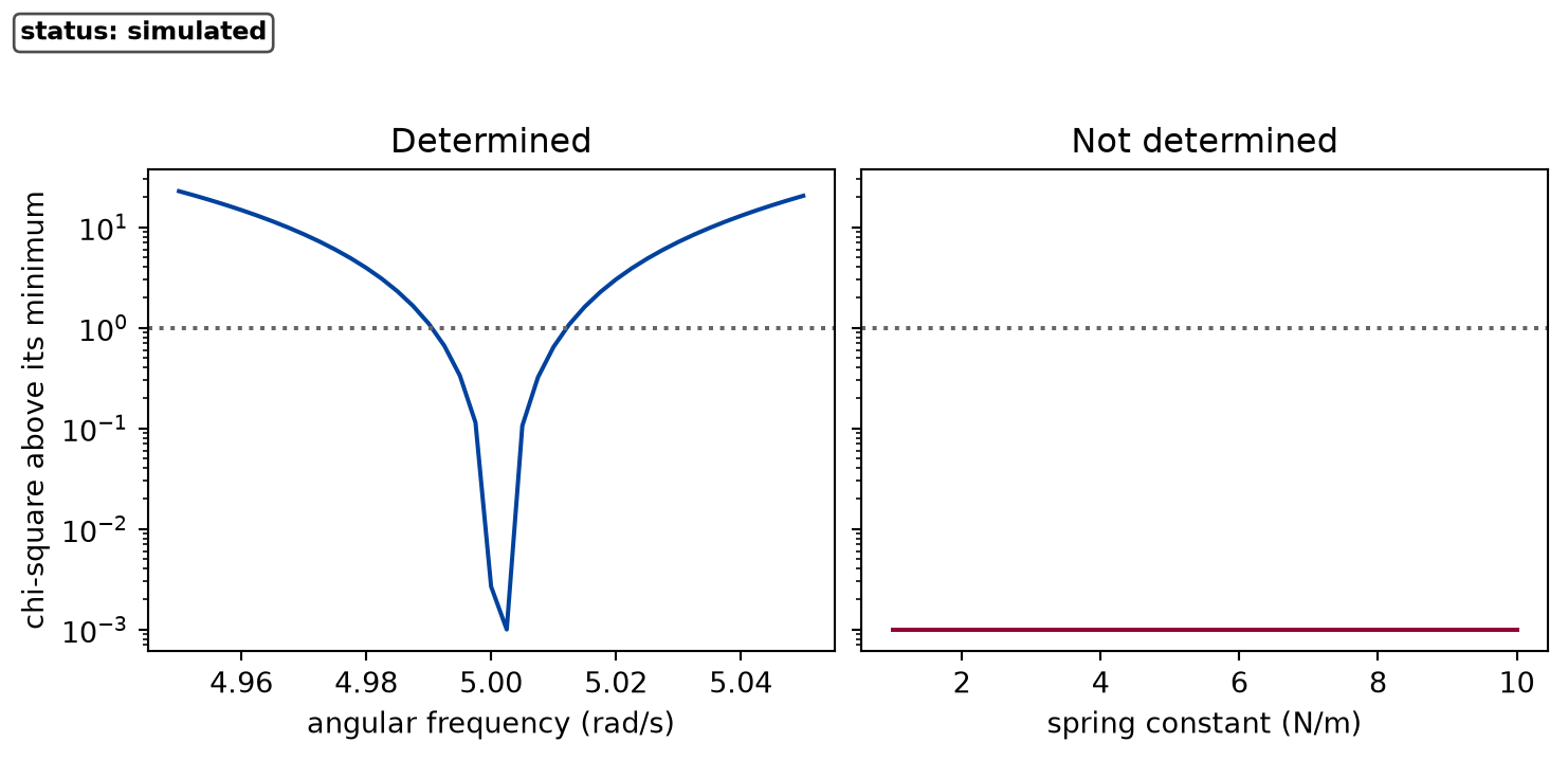
The helper reports it in two ways. The scaled Jacobian of the fit has a singular value of ratio 3e-08 between the smallest and the largest, so a combination of $k$ and $m$ is not constrained, and the standard errors of both are infinite. The profile says the same without a linear approximation: with $m$ refitted at every $k$ from 1 to 10, the chi-square never rises by more than 0.00, so the data are as happy with a spring constant of 1 as of 10.

Numerically verified (free oscillation of a mass on a spring, noise of 0.05, 120 samples): A free oscillation fitted with the mass and the spring constant as separate parameters is reported as not identified: the helper flags both parameters, and the profile of the spring constant stays within 0.0 of its minimum over a tenfold range, so no interval for either exists. The remedy is a measurement that depends on the two differently, for example a known force, or the amplitude of a forced oscillation, or a second mass added. It is a change to the experiment, not to the fit.

def frequency_profile():
    """A damped oscillation with noise, and the profile of its angular
    frequency."""
    rng = np.random.default_rng(1)
    y_damped = damped(t, *TRUTH) + rng.normal(0.0, SIGMA, t.size)
    w_grid = np.linspace(4.95, 5.05, 41)
    profile_w = profile(
        damped, t, y_damped, TRUTH, "omega", w_grid, sigma=SIGMA, names=NAMES
    )
    return y_damped, profile_w

src/pbc/mechanics/experiments/inverse_physics.py, lines 131 to 140, read from the repository when this page was built.

def draw_profiles(profile_w, profile_k) -> Figure:
    """The profile of a determined and of an undetermined parameter."""
    fig, (left, right) = plt.subplots(
        1, 2, figsize=(7.6, 3.6), sharey=True, constrained_layout=True
    )
    left.semilogy(
        profile_w.grid,
        np.maximum(profile_w.chi2 - profile_w.chi2.min(), 1e-3),
        color=FIGURE_COLOURS[0],
    )
    left.set_xlabel("angular frequency (rad/s)")
    left.set_ylabel("chi-square above its minimum")
    left.set_title("Determined")
    right.semilogy(
        profile_k.grid,
        np.maximum(profile_k.chi2 - profile_k.chi2.min(), 1e-3),
        color=FIGURE_COLOURS[1],
    )
    right.set_xlabel("spring constant (N/m)")
    right.set_title("Not determined")
    for ax in (left, right):
        ax.axhline(1.0, color="0.4", linestyle=":")
    label_status(fig, "simulated")
    return fig

src/pbc/mechanics/experiments/inverse_physics.py, lines 143 to 166, read from the repository when this page was built.

Two panels sharing a logarithmic vertical axis of chi-square above its minimum. The left panel, angular frequency, shows a narrow V-shaped bowl whose two arms rise steeply and cross a dotted horizontal line at one, a little either side of the minimum. The right panel, spring constant from one to ten, shows a flat line along the very bottom of the axis that never approaches the dotted line. — Figure 1: simulated Chi-square against one parameter, the others refitted at each value, relative to the minimum. The angular frequency of the damped oscillation has a narrow bowl; the spring constant of the free oscillation, where the mass can compensate, has a flat profile with no interval. The dotted line marks one above the minimum.

The left panel is the contrast: a parameter that the data bound, with an interval from 4.991 to 5.012 radians per second at one above the minimum.

A model that is wrong

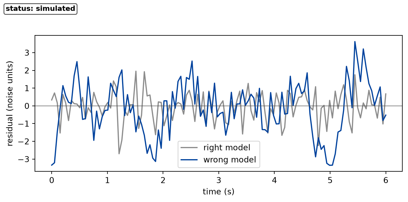
The second failure is quieter. Suppose the true damping is of dry friction, a loss that falls linearly with time, and the fit uses the exponential decay of the viscous model. The optimiser converges, the parameters have small standard errors, and the curve passes through the points to the eye. The residuals say otherwise.

def wrong_model(y_damped):
    """The damped model fitted to a linear loss and to its own data."""
    envelope = np.clip(1.0 - t / 5.0, 0.0, None)  # linear loss: dry friction
    rng = np.random.default_rng(5)
    y_dry = envelope * np.cos(5.0 * t + 0.4) + rng.normal(0.0, SIGMA, t.size)
    wrong = fit_curve(damped, t, y_dry, TRUTH, sigma=SIGMA, names=NAMES)
    right_fit = fit_curve(damped, t, y_damped, TRUTH, sigma=SIGMA, names=NAMES)
    print("wrong model, reasons against:")
    for reason in verdict(wrong):
        print(" -", reason)
    print("right model, reasons against:", verdict(right_fit) or "none")
    return wrong, right_fit

src/pbc/mechanics/experiments/inverse_physics.py, lines 169 to 180, read from the repository when this page was built.

wrong model, reasons against:
 - the residuals are correlated (lag-1 autocorrelation 0.61, 7 standard deviations from independent noise): the model leaves structure, or the noise is not independent
right model, reasons against: none

The fit of the wrong model has a reduced chi-square of 2.4 against 0.7 for the right one, and the lag-one autocorrelation of its residuals is far outside what independent noise gives. Both are consequences of one thing: the residuals still hold a smooth signal. The size of the standard errors says nothing here, because they are the errors of the parameters if the model is right.

def draw_residuals(wrong, right_fit) -> Figure:
    """The residuals of the right and of the wrong model."""
    fig, ax = plt.subplots(figsize=(7.0, 3.4), constrained_layout=True)
    ax.plot(t, right_fit.residuals / SIGMA, color="0.55", label="right model")
    ax.plot(t, wrong.residuals / SIGMA, color=FIGURE_COLOURS[0], label="wrong model")
    ax.axhline(0.0, color="0.3", lw=0.6)
    ax.set_xlabel("time (s)")
    ax.set_ylabel("residual (noise units)")
    ax.legend()
    label_status(fig, "simulated")
    return fig

src/pbc/mechanics/experiments/inverse_physics.py, lines 183 to 193, read from the repository when this page was built.

Line plot of residuals in units of the noise against time over six seconds. A grey curve scatters irregularly about zero within a band of about two units. A coloured curve makes slow swings of several samples each, away from zero and back, and reaches the largest excursions, about three units, near the start and in the last second. — Figure 2: simulated Residuals of two fits of the same kind of data, in units of the noise. With the right model (grey) they scatter about zero. With the exponential decay fitted to a linear loss (coloured) they swing in a slow pattern, which independent noise does not.

Numerically verified (one seeded data set of each kind, noise of 0.05, 120 samples): A fit of the exponentially damped oscillation to data with a linear loss converges with small standard errors and a reduced chi-square of 2.4, and the verdict of the helper lists structure in its residuals; the same fit to data of the right model lists none. A fit is evidence for a model only when it is a good fit and nothing is left in the residuals and the data determine the parameters. Each of the three can fail alone.

The measured case: the chirp mass of GW150914

The gravitational-wave lesson fitted the Newtonian chirp to the whitened strain and reported a chirp mass. The same three questions apply, and a new one that only a known signal can answer: how far is the estimate from the truth on this noise? The measured strain has no known truth, so the truth is made. A chirp of known chirp mass, the size of the fitted signal, is added to stretches of the file where no event is, and the same fit is run on each.

BAND = (35.0, 350.0)
WINDOW = (-0.2, 0.0)

src/pbc/mechanics/experiments/inverse_physics.py, lines 56 to 57, read from the repository when this page was built.

def strain_fit():
    """The chirp fitted to the committed strain of GW150914, as in the strain
    lesson."""
    gw_strains = {
        det: read_strain(SAMPLES_DIR / "gw150914-strain" / file)
        for det, file in FILES.items()
    }
    gw_rate = gw_strains["H1"].sample_rate
    gw_wide = {det: cut_segment(s, 2.0) for det, s in gw_strains.items()}
    gw_white = {
        det: make_whitener(gw_strains[det], gw_wide[det], BAND)(gw_wide[det].strain)
        for det in gw_strains
    }
    gw_corr = correlation_with_control(
        gw_white["H1"], gw_white["L1"], gw_wide["H1"].time, gw_rate
    )
    gw_delays = {"H1": 0.0, "L1": gw_corr["lag"]}

    gw_seg = {det: cut_segment(s, 0.75) for det, s in gw_strains.items()}
    gw_time = gw_seg["H1"].time
    gw_whiteners = {
        det: make_whitener(gw_strains[det], gw_seg[det], BAND) for det in gw_strains
    }
    gw_data = {det: gw_whiteners[det](gw_seg[det].strain) for det in gw_strains}
    gw_sigma = noise_sigma(gw_data["H1"], gw_time, (0.3, 0.65))
    gw_fit = fit_chirp(
        gw_time,
        gw_data,
        gw_whiteners,
        gw_delays,
        window=WINDOW,
        sigma=gw_sigma,
        mc_grid=np.arange(22.0, 50.0, 1.0),
    )
    gw_inside = (gw_time >= WINDOW[0]) & (gw_time <= WINDOW[1])
    gw_peak = {
        det: float(np.max(np.abs(gw_fit.models[det][gw_inside]))) for det in gw_strains
    }
    return gw_strains, gw_delays, gw_seg, gw_time, gw_data, gw_fit, gw_peak

src/pbc/mechanics/experiments/inverse_physics.py, lines 196 to 234, read from the repository when this page was built.

The reasons against taking this fit as evidence, from the same helper: the data do not determine chirp mass separately (a combination of them is not constrained); the residuals are correlated (lag-1 autocorrelation 0.95, 38 standard deviations from independent noise): the model leaves structure, or the noise is not independent. The fit gives a chirp mass of 41.0 solar masses with a profile interval of 40.8 to 42.0, and a reduced chi-square of 0.85.

Both reasons deserve a reading. The first is the tie of the chirp mass with the coalescence time that the gravitational-wave lesson described: the interval of the profile, and not the standard error of the covariance, is the statement about the mass. The second is a property of the processing before it is a property of the model. The whitened strain was band-passed, which makes neighbouring samples alike even for noise alone. The next cell measures that on a stretch of the whitened strain with no event, and then runs the injection.

def noise_correlation(gw_time, gw_data):
    """The correlation of neighbouring samples of the whitened noise."""
    quiet = (np.abs(gw_time) > 0.3) & (np.abs(gw_time) < 0.65)
    return residual_autocorrelation(gw_data["H1"][quiet])[0]

src/pbc/mechanics/experiments/inverse_physics.py, lines 237 to 240, read from the repository when this page was built.

The lag-one autocorrelation of the whitened Hanford noise away from the event is 0.95, close to that of the residuals, so the helper’s second reason is in large part the band-pass and not a missing piece of the model. It does mean that the samples are not independent, which the stated interval assumes.

TRUTH_MC, TRUTH_TC = 35.0, 0.03
CENTRES = [-12.0, -8.0, 8.0, 12.0]  # seconds from the event: no event there

src/pbc/mechanics/experiments/inverse_physics.py, lines 60 to 61, read from the repository when this page was built.

def injection(experiment: Experiment, gw_strains, gw_delays, gw_peak):
    """A known chirp added to four stretches of strain without an event and
    fitted; record the table."""
    injections = inject_and_fit(
        gw_strains,
        CENTRES,
        truth_mc=TRUTH_MC,
        truth_tc=TRUTH_TC,
        delays=gw_delays,
        peak=gw_peak,
        band=BAND,
        window=WINDOW,
        mc_grid=np.arange(24.0, 48.0, 1.0),
    )
    inj_mc = np.array([inj.mc for inj in injections])
    inj_half = float(np.mean([(inj.high - inj.low) / 2 for inj in injections]))
    inj_rms = float(np.sqrt(np.mean((inj_mc - TRUTH_MC) ** 2)))
    inj_worst = float(np.max(np.abs(inj_mc - TRUTH_MC)))
    inj_covered = sum(inj.covers(TRUTH_MC) for inj in injections)
    experiment.table(
        "injection",
        [
            (
                inj.centre,
                inj.mc,
                inj.low,
                inj.high,
                "yes" if inj.covers(TRUTH_MC) else "no",
            )
            for inj in injections
        ],
        columns=[
            ("noise taken around", "s from the event", ".0f"),
            ("recovered chirp mass", "solar masses", ".1f"),
            ("stated interval, low", "solar masses", ".1f"),
            ("stated interval, high", "solar masses", ".1f"),
            ("holds the truth", "", "s"),
        ],
        caption=f"A chirp of {TRUTH_MC:g} solar masses, of the size of the fitted "
        "signal, added to four stretches of strain without an event.",
    )
    return len(injections), inj_half, inj_rms, inj_worst, inj_covered

src/pbc/mechanics/experiments/inverse_physics.py, lines 243 to 284, read from the repository when this page was built.

A chirp of 35 solar masses, of the size of the fitted signal, added to four stretches of strain without an event.
noise taken around (s from the event)	recovered chirp mass (solar masses)	stated interval, low (solar masses)	stated interval, high (solar masses)	holds the truth
-12	35.1	34.9	35.4	yes
-8	35.0	34.7	35.1	yes
8	36.0	35.8	36.1	no
12	35.0	35.0	35.1	yes

The injected chirp is recovered: the estimates lie within 1.0 solar masses of the truth. But the stated intervals, 0.2 solar masses wide on average on each side, hold the truth in only 3 of 4 stretches, while the root-mean-square error of the estimates is 0.5 solar masses. The interval of the profile assumes independent noise, which the real noise is not, and here it is too small. The scatter of the injections points more directly at the uncertainty due to the noise, but four stretches are a demonstration and not an estimate: they show that the interval is too small, not how large it should be.

def band_spread(gw_strains, gw_delays, gw_seg, gw_time, gw_fit):
    """The chirp mass for three bands of the fit."""
    gw_bands = [(35.0, 350.0), (35.0, 250.0), (30.0, 300.0)]
    gw_band_mc = []
    for band in gw_bands:
        if band == BAND:
            gw_band_mc.append(gw_fit.mc)
            continue
        whiten = {
            det: make_whitener(gw_strains[det], gw_seg[det], band) for det in gw_strains
        }
        gw_series = {det: whiten[det](gw_seg[det].strain) for det in gw_strains}
        other = fit_chirp(
            gw_time,
            gw_series,
            whiten,
            gw_delays,
            window=WINDOW,
            sigma=noise_sigma(gw_series["H1"], gw_time, (0.3, 0.65)),
            mc_grid=np.arange(26.0, 48.0, 2.0),
        )
        gw_band_mc.append(other.mc)
    return min(gw_band_mc), max(gw_band_mc)

src/pbc/mechanics/experiments/inverse_physics.py, lines 287 to 309, read from the repository when this page was built.

    gw_spread = band_spread(gw_strains, gw_delays, gw_seg, gw_time, gw_fit)
    gw_half = (gw_fit.mc_high - gw_fit.mc_low) / 2
    gw_excess = gw_fit.mc - gw_published

src/pbc/mechanics/experiments/inverse_physics.py, lines 442 to 444, read from the repository when this page was built.

The noise is one source of uncertainty, and the choice of analysis is another. Repeating the fit with three bands, as the earlier lesson did, gives chirp masses from 38 to 41 solar masses.

Experimentally supported (Newtonian-order chirp, window of 0.2 s before the event time, four off-source stretches, three bands, noise estimated from the file): The fit of the Newtonian chirp to the measured strain gives a detector-frame chirp mass of 41 solar masses with a profile interval of 0.6 on each side. A known chirp of 35 solar masses added to four stretches of strain without an event is recovered with a root-mean-square error of 0.5 solar masses where the stated intervals averaged 0.2, and the choice of band moves the fitted value between 38 and 41; the estimate is 10 solar masses above the published detector-frame value of 31. The uncertainty to quote for the measured value is therefore not the interval of the profile. It is at least the scatter that the injections show, and the spread over the analysis is larger still; neither contains the error of the model, which the earlier lesson lists among the possible reasons for the distance to the published value and which this lesson does not measure.

What the fit cannot say

The fit has two parameters, the chirp mass and the coalescence time, and the singular ratio of 1.6e-05 of the helper shows how close to tied they are. A different identifiability limit sits in the model itself. At leading order the chirp depends on the masses only through $\mathcal{M}$ , so every pair of masses with that chirp mass fits equally well:

def degenerate_masses(experiment: Experiment, gw_fit) -> None:
    """Pairs of masses with the chirp mass of the fit; record the table."""
    mass_rows = []
    for q in (1.0, 0.8, 0.5, 0.25):
        # m1 + m2 from the chirp mass at a given ratio q = m2 / m1.
        total_mass = gw_fit.mc * (1 + q) ** (6 / 5) / q ** (3 / 5)
        heavier = total_mass / (1 + q)
        mass_rows.append(
            (q, heavier, q * heavier, float(chirp.chirp_mass(heavier, q * heavier)))
        )
    experiment.table(
        "degenerate-masses",
        mass_rows,
        columns=[
            ("mass ratio", "", ".2f"),
            ("heavier mass", "solar masses", ".0f"),
            ("lighter mass", "solar masses", ".0f"),
            ("chirp mass", "solar masses", ".1f"),
        ],
        caption="Pairs of masses with the chirp mass of the fit: the leading-order "
        "chirp is the same for all of them.",
    )

src/pbc/mechanics/experiments/inverse_physics.py, lines 312 to 333, read from the repository when this page was built.

Pairs of masses with the chirp mass of the fit: the leading-order chirp is the same for all of them.
mass ratio	heavier mass (solar masses)	lighter mass (solar masses)	chirp mass (solar masses)
1.00	47	47	41.0
0.80	53	42	41.0
0.50	67	34	41.0
0.25	99	25	41.0

The four pairs differ in the heavier mass by a large factor and give the same chirp, so the data of this model constrain no individual mass. A statement of the two masses from this fit would be an answer to a question the model cannot ask, exactly like the spring constant above.

Limits

Synthetic recovery is a test of the procedure. It shows that the fit works when its assumptions hold. The injection of the last section is closer to the real case because the noise is real, but the injected signal is the model itself, so it cannot show an error of the model.
The standard errors and the profile assume the noise is white. The injection shows by how much they fail in the measured case; four stretches give the scatter only roughly, and a different seed or more stretches would change the number.
The verdict is a screen. It looks for the three failures of the lesson. A residual structure of the size of the noise, a model that is wrong in a way the data cannot show, or an identifiable parameter that is simply biased, pass it.
The sloppy-direction threshold is a convention. The helper calls a combination undetermined below a singular ratio of $10^{-4}$ . A ratio of $10^{-3}$ is a weakly determined parameter with a large error bar, and nothing in the helper says where the border is for a given purpose.
The measured case is one event and one model. The comparison with the published value is a statement about this method on this record, not a test of the theory.
No agent is part of this lesson. The roadmap allows an agent that proposes fits; it is not built here, and the helpers do not depend on one.

In plain words: a fit hands back numbers whatever the data hold. Run it first on data whose answer you know, ask whether the data can separate the parameters, look at what the residuals still contain, and quote the uncertainty that the known-signal test shows rather than the one the optimiser prints.

Self-check. A fit of $x(t) = a\,b\,\sin(\omega t)$ with $a$ and $b$ both free returns small standard errors for $\omega$ and a perfect-looking curve. What should you report for $a$ and $b$ , and what would make them separately measurable?

With scripts, you can record in this browser that you answered this question.

Solution to the self-check

Nothing for $a$ and $b$ separately: they appear only as the product $ab$ , so the helper flags both as not identified and their profiles are flat. Report the product $ab$ with its error. They become measurable if another observation depends on them differently, for instance a second quantity that contains $a$ alone.

Exercises

Exercise 1. A record that is too short. Run recover on the damped oscillation with the times np.linspace(0, 0.8, 30) and sigma=0.2, so that the record covers less than a decay time. Which parameter is determined worst compared with its own size, and do the stated errors still follow the scatter?

Hint 1 of 1 for exercise 1

Divide the rms_error of each parameter by its truth, and compare rms_error with mean_stderr.

Solution to exercise 1

def short_record(experiment: Experiment) -> None:
    """Exercise 1: fits of a record shorter than one decay time; record the
    table."""
    t_short = np.linspace(0.0, 0.8, 30)
    short = recover(damped, t_short, TRUTH, sigma=0.2, trials=100, seed=4, names=NAMES)
    rows = [
        (label, rms / value, stated, rms, 100 * cover)
        for label, value, cover, rms, stated in zip(
            short.names,
            short.truth,
            short.coverage,
            short.rms_error,
            short.mean_stderr,
            strict=True,
        )
    ]
    experiment.table(
        "short-record",
        rows,
        columns=[
            ("parameter", "", "s"),
            ("scatter over value", "", ".2f"),
            ("stated error", "", ".3f"),
            ("scatter", "", ".3f"),
            ("coverage", "%", ".0f"),
        ],
        caption="Fits of a record shorter than one decay time: the stated error "
        "against the scatter of 100 trials.",
    )

src/pbc/mechanics/experiments/inverse_physics.py, lines 336 to 364, read from the repository when this page was built.

Fits of a record shorter than one decay time: the stated error against the scatter of 100 trials.
parameter	scatter over value	stated error	scatter	coverage (%)
amplitude	0.16	0.168	0.157	95
decay	0.99	0.371	0.345	97
omega	0.07	0.374	0.356	94
phase	0.36	0.143	0.142	95

The decay is the worst: in a record shorter than one decay time the amplitude barely falls, so the rate has a scatter as large as its value. The stated errors still follow the scatter, which is why a wide stated error is honest here, and why a result with a standard error as large as the value is not a measurement.

Exercise 2. A second mass. Add a second parameter set to the spring: a known extra mass of 0.5 added to the moving mass in a second run, with the same spring. Fit both runs together for $k$ and $m$ and show that they are now determined.

Hint 1 of 1 for exercise 2

The combined model concatenates the two runs; each has its own $\omega$ . Use fit_curve on the concatenated times and look at identifiable.

Solution to exercise 2

def two_runs(index, k, m):
    first = np.cos(np.sqrt(k / m) * t)
    second = np.cos(np.sqrt(k / (m + 0.5)) * t)
    return np.where(
        index < t.size,
        first[np.minimum(index, t.size - 1).astype(int)],
        second[np.maximum(index - t.size, 0).astype(int)],
    )

src/pbc/mechanics/experiments/inverse_physics.py, lines 367 to 374, read from the repository when this page was built.

def joint_fit():
    """Exercise 2: k and m from two runs, the second with a known extra
    mass."""
    index = np.arange(2 * t.size, dtype=float)
    rng = np.random.default_rng(8)
    y_two = two_runs(index, K_TRUE, M_TRUE) + rng.normal(0.0, SIGMA, index.size)
    joint = fit_curve(
        two_runs, index, y_two, [4.5, 1.1], sigma=SIGMA, names=["k", "m"], bounds=bound
    )
    print("identifiable:", joint.identifiable)
    print(
        f"k = {joint.value('k'):.2f} +/- {joint.stderr[0]:.2f},"
        f" m = {joint.value('m'):.2f} +/- {joint.stderr[1]:.2f}"
    )

src/pbc/mechanics/experiments/inverse_physics.py, lines 377 to 390, read from the repository when this page was built.

identifiable: (True, True)
k = 4.06 +/- 0.03, m = 1.02 +/- 0.01

Changing the experiment gave the fit what it lacked.

Run this experiment

This page was built from commit 6417e2ff90258bd2d2ba21d217eb7666fd24f680 of the repository.

In a clone at that commit, with the project’s Python packages installed, this command runs the experiment of this page:

uv run --locked --no-dev python -m pbc.mechanics.experiments.inverse_physics results

Files, tests, and every command

The files behind it:

site/lessons/mechanics/12-inverse-physics-parameter-discovery/index.qmd: this page, with every code cell.
src/pbc/data/fit.py: code the experiment runs.
src/pbc/data/inverse.py: code the experiment runs.
src/pbc/data/gwinjection.py: code the experiment runs.
src/pbc/data/gwstrain.py: code the experiment runs.
src/pbc/mechanics/chirp.py: code the experiment runs.
src/pbc/mechanics/experiments/inverse_physics.py: code the experiment runs.
src/pbc/experiment.py: code the experiment runs.
tests/unit/test_inverse.py: tests of that code.
tests/unit/test_gwstrain.py: tests of that code.
tests/unit/test_data_analysis.py: tests of that code.
tests/unit/test_inverse_physics_experiment.py: tests of that code.

With Git and uv installed (see the setup page), run:

git clone https://github.com/taspinar/physics-by-construction.git
cd physics-by-construction
git checkout 6417e2ff90258bd2d2ba21d217eb7666fd24f680
uv sync --locked --no-dev
uv run --locked --no-dev python -m pbc.mechanics.experiments.inverse_physics results

The experiment writes every figure of this page into results/, as <label>.png, and every number and table of the page, as the page shows it, into results/results.json. Its numbers match this page to the digits shown, and its figure files are the ones the page shows; digits beyond those can differ between machines, because floating-point libraries differ. Change the code of the experiment and run it again to see what changes.