Double pendulum and chaos

Two rods hung from each other: a motion that is regular at small angles and chaotic at large ones, told apart by how fast two nearly identical starts separate, and measured by an estimate of the Lyapunov exponent that is checked against its expected sign in both regimes.

Course

Classical mechanics, lesson 9 of 28

Slot

M9, Double pendulum and chaos

Methods

Simulation

Difficulty

Advanced, level 3 of 3

What you’ll learn

Simulate the double pendulum and check it against its small-oscillation modes and its energy
Measure how two nearly identical starts separate, in a regular and in a chaotic motion
Estimate the largest Lyapunov exponent and say what its sign means
State how long a chaotic motion can be predicted, and what a finer step does and does not change

Prerequisites

Energy conservation, Numerical integrators.

Before you begin

Calculus: the chain rule, and the exponential function as the solution of a rate proportional to the amount
Trigonometry: the sine and cosine of a difference of angles
Logarithms: the natural logarithm of a ratio, and its use to read a growth rate from a straight line on a logarithmic axis
Linear algebra: the Euclidean norm of a vector

Related

Lagrangian mechanics

Previous

Inverse physics: parameters from observations

Next

Lagrangian mechanics

With scripts, this page keeps a record in your browser of whether you completed the lesson. Nothing is stored without them.

With scripts, this place suggests what to do next, with the reason, from the progress saved in your browser. Without them, follow the learning path.

Hang a second rod from the end of a pendulum, with a bob on each, and let the two swing in a vertical plane. Nothing in the setup is random: two masses, two rods, gravity, and the same laws as in every lesson before this one. Yet release it from a large angle twice, with the second start differing from the first by less than a hair’s breadth, and for a while the two swings are the same and then they are not. The motion is deterministic and it cannot be predicted for long, and the same is true of weather, of the tumbling of bodies in orbit, and of a drop of dye in a stirred liquid. The question of the lesson is how to measure that, and how to tell a motion that is only complicated from one that is chaotic.

The measure is the rate at which two nearby starts move apart: the Lyapunov exponent. The lesson builds the double pendulum on the stepping interface of the earlier lessons, trusts it for two independent reasons (the frequencies of its small oscillations and its energy), watches the separation of two starts in a regular and in a chaotic regime, and turns that into an estimate whose sign is checked in both. It ends with what the number does not say.

Assumptions

The model and the program rest on these assumptions. Each one names what goes wrong when it does not hold.

Two rigid, massless rods in a plane, with point bobs. Two angles describe the configuration, and the tensions in the rods do no work. A rod with mass, a bob of finite size, or a swing out of the plane (a spherical double pendulum) is a different system with a different number of coordinates.
No friction at the joints and no drag. The energy is conserved and the motion never settles. With friction the motion decays onto the hanging rest position and has no chaos left to measure.
Constant gravity and constant lengths. The weights are uniform and the rods do not stretch.
The equations are those of the Lagrangian lesson. They are given here, and two checks stand in for the derivation: the frequencies of the small oscillations, and the energy. The next lesson derives them from one function and compares them with the program.
The step resolves the motion. The classical Runge-Kutta method with a step far below the fastest time scale of the pendulum keeps the energy within a small bound for the runs here. A chaotic run amplifies every error of the step, so a trajectory of a given run is the trajectory of the method and that step, not an exact one; what can be trusted is a statistical property of the motion, such as the exponent, and the short time before errors have grown.
The separation is small. The estimate follows two starts that differ by a distance far smaller than the motion itself, and puts them back together before the difference stops being small. A separation as large as the motion measures the size of the region the motion fills, not the exponent.

The double pendulum and the exponent

The equations of motion

Let $\theta_1$ be the angle of the first rod from the downward vertical, and $\theta_2$ the angle of the second rod from the same line. The bobs have the masses $m_1$ and $m_2$ and the rods the lengths $l_1$ and $l_2$ . The state of the program is the pair of angles as the position and the pair of angular velocities as the velocity, the same layout as the one-coordinate pendulum of the energy lesson with two entries instead of one.

With $\Delta = \theta_1 - \theta_2$ the energy is

$E = \tfrac12 (m_1 + m_2)\, l_1^2\,\dot\theta_1^2 + \tfrac12 m_2\, l_2^2\,\dot\theta_2^2 + m_2\, l_1 l_2\, \dot\theta_1 \dot\theta_2 \cos\Delta - (m_1 + m_2)\, g\, l_1 \cos\theta_1 - m_2\, g\, l_2 \cos\theta_2 .$

The cross term is why the double pendulum is not two pendulums side by side: the velocity of the second bob is the velocity of the first plus its own, and the kinetic energy of the sum has a product of the two angular velocities. The angular accelerations that follow, from the Lagrangian of the next lesson, are

$\ddot\theta_1 = \frac{-g(2m_1 + m_2)\sin\theta_1 - m_2 g \sin(\theta_1 - 2\theta_2) - 2\sin\Delta\; m_2\,(\dot\theta_2^2 l_2 + \dot\theta_1^2 l_1\cos\Delta)} {l_1\,(2m_1 + m_2 - m_2\cos 2\Delta)},$

$\ddot\theta_2 = \frac{2\sin\Delta\,\bigl(\dot\theta_1^2 l_1 (m_1 + m_2) + g(m_1 + m_2)\cos\theta_1 + \dot\theta_2^2 l_2 m_2\cos\Delta\bigr)} {l_2\,(2m_1 + m_2 - m_2\cos 2\Delta)} .$

Both have the same denominator, which is the determinant of the matrix that multiplies the accelerations, and it never vanishes for positive masses. Nothing here is checked by being displayed. Two facts that can be computed check it. For small angles the sines and cosines can be linearised and the motion is a sum of two normal modes; for equal masses and equal rods their squared angular frequencies are

$\omega_\pm^2 = \frac{g}{l}\,(2 \pm \sqrt 2),$

the slower with the two bobs swinging together (the outer angle $\sqrt 2$ times the inner), the faster with them against each other. And the energy above must stay constant along a simulated motion, to the accuracy the earlier lessons established for the method.

Sensitivity to the start

Take a start and a second start that differs from it by a small vector $\delta_0$ in the combined space of the two angles and the two angular velocities, and follow both. Let $d(t)$ be the length of the difference. While it is small the difference obeys the linearised equations of motion, so its growth does not depend on its size. In a regular motion it grows slowly, as a power of the time. In a chaotic motion it grows exponentially,

$d(t) \approx d_0\, e^{\lambda t}, \qquad \lambda = \lim_{t \to \infty}\; \lim_{d_0 \to 0}\; \frac1t \ln\frac{d(t)}{d_0},$

and $\lambda$ , with the unit one per second, is the largest Lyapunov exponent. The sign says what kind of motion it is. A positive exponent means that any error in the start, however small, is multiplied by a factor of $e$ every $1/\lambda$ seconds. Zero means that errors grow at most as a power of time, as in the regular swing of a small oscillation. The exponent is a property of the motion and not of the pair of starts, for almost every pair.

The consequence is a predictability horizon. If the start is known to a distance $d_0$ and a prediction is useful while the error stays below $\Delta$ (both measured as the distance in phase space, with the equal-weight metric of the estimate below, so $\Delta$ in the same units), the useful time is

$t_h \approx \frac1\lambda \ln\frac{\Delta}{d_0}.$

It is a logarithm of the accuracy of the start: a measurement a million times better buys only the same few extra $1/\lambda$ of useful prediction, once.

How the exponent is estimated

The definition needs an infinitely small separation and an infinite time, and a program has neither. The estimate follows the pair of starts for a time $\tau$ , measures the length $d_1$ of their difference, adds $\ln(d_1/d_0)$ to a running sum, and then moves the second start back along the line to the first until their distance is $d_0$ again. It repeats the rescaling to the end of the run, and the estimate is the sum divided by the time. The rescaling does two things: it keeps the separation inside the range where the linearised growth holds, and it keeps it from reaching the size of the whole region the motion fills, where it cannot grow any more. A single separation that is allowed to grow measures that size after a short while, and gives an exponent that falls to zero with the time whatever the motion.

A finite run gives a finite-time estimate. In a regular motion its value falls as the run lengthens, roughly as one over the time, towards zero. In a chaotic motion it settles near a positive value and varies a little from one trajectory to another. Whether a run belongs to one or the other is read from that behaviour, not from one number.

The program

The reusable code is pbc.mechanics.chaos. The double pendulum is an acceleration in the sense of the stepping interface, so every stepper of the earlier lessons applies to it unchanged.

def double_pendulum(
    m1: float, m2: float, l1: float, l2: float, g: float = STANDARD_GRAVITY
) -> Acceleration:
    """The angular accelerations (rad/s²) of a double pendulum with the bob
    masses ``m1`` and ``m2`` (kg) on rods of length ``l1`` and ``l2`` (m).

    The position is the pair of angles of the rods from the downward vertical,
    the velocity the pair of angular velocities. The equations come from the
    Lagrangian; the denominator is the determinant of the mass matrix, which
    never vanishes for positive masses.
    """
    if min(m1, m2, l1, l2, g) <= 0:
        raise ValueError("masses, lengths, and g must be positive")

    def acceleration(t: float, x: Vector, v: Vector) -> Vector:
        delta = x[0] - x[1]
        sin_d, cos_d = np.sin(delta), np.cos(delta)
        den = 2.0 * m1 + m2 - m2 * np.cos(2.0 * delta)
        a1 = (
            -g * (2.0 * m1 + m2) * np.sin(x[0])
            - m2 * g * np.sin(x[0] - 2.0 * x[1])
            - 2.0 * sin_d * m2 * (v[1] ** 2 * l2 + v[0] ** 2 * l1 * cos_d)
        ) / (l1 * den)
        a2 = (
            2.0
            * sin_d
            * (
                v[0] ** 2 * l1 * (m1 + m2)
                + g * (m1 + m2) * np.cos(x[0])
                + v[1] ** 2 * l2 * m2 * cos_d
            )
        ) / (l2 * den)
        return np.array([a1, a2])

    return acceleration

Line 48, den = 2.0 * m1 + m2 - m2 * np.cos(2.0 * delta): The denominator both accelerations share: the determinant of the mass matrix, positive for positive masses.
Line 63, return np.array([a1, a2]): The two angular accelerations, in the order of the angles, in radians per second squared.

src/pbc/mechanics/chaos.py, lines 31 to 65, read from the repository when this page was built.

The energy of the pendulum, with the cross term of the two angular velocities:

def double_pendulum_energy(
    x: NDArray[np.float64],
    v: NDArray[np.float64],
    m1: float,
    m2: float,
    l1: float,
    l2: float,
    g: float = STANDARD_GRAVITY,
) -> NDArray[np.float64]:
    """The energy in J of a double pendulum at every row of the angles ``x``
    (rad) and angular velocities ``v`` (rad/s), arrays of shape (n, 2).

    The kinetic energy has a cross term of the two angular velocities, so it
    is not the sum of two single-pendulum energies.
    """
    x, v = np.atleast_2d(x), np.atleast_2d(v)
    kinetic = (
        0.5 * (m1 + m2) * l1**2 * v[:, 0] ** 2
        + 0.5 * m2 * l2**2 * v[:, 1] ** 2
        + m2 * l1 * l2 * v[:, 0] * v[:, 1] * np.cos(x[:, 0] - x[:, 1])
    )
    potential = -(m1 + m2) * g * l1 * np.cos(x[:, 0]) - m2 * g * l2 * np.cos(x[:, 1])
    return kinetic + potential

src/pbc/mechanics/chaos.py, lines 68 to 90, read from the repository when this page was built.

The estimate of the exponent, with the rescaling of the second start:

def lyapunov_exponent(
    initial: State,
    acceleration: Acceleration,
    dt: float,
    n_steps: int,
    separation: float = 1e-8,
    rescale_every: int = 10,
    step: Stepper = rk4_step,
) -> LyapunovEstimate:
    """Estimate the largest Lyapunov exponent (1/s) of the motion from
    ``initial`` by following a second trajectory that starts ``separation``
    away in phase space.

    The distance is the Euclidean norm of the difference of the combined
    vector of positions (rad) and velocities (rad/s), with equal weight, so
    the metric implicitly measures time in units of 1 s: a velocity
    difference of 1 rad/s counts as much as an angle difference of 1 rad.
    The exponent does not depend on this choice, but the finite-time
    separation does. Every ``rescale_every`` steps of
    length ``dt`` (s) the logarithm of the growth of the distance is added up
    and the second trajectory is pulled back to ``separation`` along the
    direction it has grown in, so the separation stays small enough to follow
    the linearised motion. The exponent is the sum of the logarithms divided
    by the time. For a regular motion the estimate falls towards zero as the
    run gets longer; for a chaotic one it settles at a positive value.
    """
    if separation <= 0 or rescale_every < 1 or n_steps < rescale_every:
        raise ValueError("need a positive separation and n_steps >= rescale_every >= 1")
    n = len(initial.x)
    first = initial
    direction = np.ones(2 * n) / np.sqrt(2 * n)
    second = State(
        t=initial.t,
        x=initial.x + separation * direction[:n],
        v=initial.v + separation * direction[n:],
    )
    total, times, running = 0.0, [], []
    for i in range(1, n_steps + 1):
        first = step(first, acceleration, dt)
        second = step(second, acceleration, dt)
        if i % rescale_every == 0:
            gap = np.concatenate([second.x - first.x, second.v - first.v])
            distance = float(np.linalg.norm(gap))
            total += np.log(distance / separation)
            gap *= separation / distance
            second = State(t=second.t, x=first.x + gap[:n], v=first.v + gap[n:])
            times.append(first.t - initial.t)
            running.append(total / (first.t - initial.t))
    return LyapunovEstimate(
        exponent=running[-1], t=np.array(times), running=np.array(running)
    )

Line 145, total += np.log(distance / separation): The growth since the last rescaling, as a logarithm, added to a running sum. Logarithms add where the growth factors multiply.
Line 146, gap *= separation / distance: The rescaling: the same direction, the original distance, so the second start stays near the first.
Line 149, running.append(total / (first.t - initial.t)): The estimate so far, in one per second: the sum divided by the time. The list shows how the estimate settles, or does not.

src/pbc/mechanics/chaos.py, lines 102 to 152, read from the repository when this page was built.

Worked examples

Two checks of the equations

The pendulum of the examples has equal masses of one kilogram and rods of one metre. The first check starts the pendulum in the slow and in the fast normal mode, with an amplitude small enough for the linear theory, and measures the period from the passages of the first angle through zero, interpolated within the step. The second runs the pendulum from a regular and from a chaotic start and reports the drift of the energy.

mass, length = 1.0, 1.0  # kg, m
pendulum = double_pendulum(mass, mass, length, length)
dt = 0.01  # s

src/pbc/mechanics/experiments/double_pendulum_chaos.py, lines 30 to 32, read from the repository when this page was built.

def released(first, second):
    """At rest, with the two rods at the given angles (rad)."""
    return State(t=0.0, x=[first, second], v=[0.0, 0.0])

src/pbc/mechanics/experiments/double_pendulum_chaos.py, lines 39 to 41, read from the repository when this page was built.

def run_for(start, duration):
    return simulate(start, pendulum, dt, round(duration / dt), step=rk4_step)

src/pbc/mechanics/experiments/double_pendulum_chaos.py, lines 44 to 45, read from the repository when this page was built.

def periods(trajectory):
    """The times between the passages of the first angle through zero in the
    same direction, interpolated within the step (s)."""
    s, t = trajectory.x[:, 0], trajectory.t
    before = np.where((s[:-1] > 0) & (s[1:] <= 0))[0]
    crossings = t[before] + s[before] / (s[before] - s[before + 1]) * (
        t[before + 1] - t[before]
    )
    return np.diff(crossings)

src/pbc/mechanics/experiments/double_pendulum_chaos.py, lines 48 to 56, read from the repository when this page was built.

def modes_and_energy(experiment: Experiment) -> None:
    """The periods of the two normal modes of small oscillations, closed form
    and simulated; record the table."""
    rows = []
    for label, ratio, factor in (
        ("slow mode", np.sqrt(2.0), 2.0 - np.sqrt(2.0)),
        ("fast mode", -np.sqrt(2.0), 2.0 + np.sqrt(2.0)),
    ):
        small = 1e-3  # rad
        trajectory = run_for(released(small, small * ratio), 12.0)
        analytic = 2.0 * np.pi / np.sqrt(g / length * factor)
        rows.append((label, analytic, np.mean(periods(trajectory))))

    experiment.table(
        "modes-and-energy",
        rows,
        columns=[
            ("mode", "", ""),
            ("period from the equations", "s", ".4f"),
            ("simulated period", "s", ".4f"),
        ],
        caption="Period of the two normal modes of the small oscillations: the "
        "closed form and the simulation, to four decimals.",
    )

src/pbc/mechanics/experiments/double_pendulum_chaos.py, lines 59 to 82, read from the repository when this page was built.

Period of the two normal modes of the small oscillations: the closed form and the simulation, to four decimals.
mode	period from the equations (s)	simulated period (s)
slow mode	2.6215	2.6215
fast mode	1.0859	1.0859

Numerically verified (equal masses and rods, amplitude of one thousandth of a radian, classical Runge-Kutta method): The simulated periods of both modes agree with the closed form to the four digits shown, so the accelerations carry the right linear part: the restoring torques, the coupling of the two rods, and the factor $\sqrt 2$ that separates the modes. The nonlinear terms, which decide the chaos, are not tested by a linear check. The energy is the second check, and it sees them:

def drift(trajectory):
    energy = double_pendulum_energy(
        trajectory.x, trajectory.v, mass, mass, length, length
    )
    return np.max(np.abs(energy - energy[0])) / abs(energy[0])

src/pbc/mechanics/experiments/double_pendulum_chaos.py, lines 85 to 89, read from the repository when this page was built.

regular_start, chaotic_start = released(0.2, 0.2), released(2.0, 2.0)

src/pbc/mechanics/experiments/double_pendulum_chaos.py, line 93, read from the repository when this page was built.

def energy_drift(experiment: Experiment):
    """Fifty seconds of a regular and a chaotic start; record the table of
    their energy drift and return the runs."""
    regular_run, chaotic_run = (
        run_for(regular_start, 50.0),
        run_for(chaotic_start, 50.0),
    )

    experiment.table(
        "energy-drift",
        [
            ("regular", 0.2, drift(regular_run)),
            ("chaotic", 2.0, drift(chaotic_run)),
        ],
        columns=[
            ("start", "", ""),
            ("both angles", "rad", ".1f"),
            ("energy drift over 50 s", "", ".1e"),
        ],
        caption="Relative energy drift of the double pendulum released at rest "
        "with both rods at the same angle, over fifty seconds, classical "
        "Runge-Kutta method.",
    )
    return regular_run, chaotic_run

src/pbc/mechanics/experiments/double_pendulum_chaos.py, lines 97 to 120, read from the repository when this page was built.

Relative energy drift of the double pendulum released at rest with both rods at the same angle, over fifty seconds, classical Runge-Kutta method.
start	both angles (rad)	energy drift over 50 s
regular	0.2	1.7e-09
chaotic	2.0	5.8e-04

Numerically verified (the two starts of the table, fifty seconds, classical Runge-Kutta method with the stated step): The energy stays within a small fraction of its start in both regimes, but the drift is 3e+05 times larger in the chaotic run. The energy drift of the method grows where the motion is violent, and this is the first sign that the program is not as exact in the chaotic regime as in the regular one.

Two starts that differ by a hair

The cell starts a second pendulum one hundred-millionth of a radian away in the first angle and follows both for thirty seconds. The separation is the length of the difference of the four-component states: two angles in radians and two angular velocities in radians per second, with equal weight, so the distance is in units that measure time in seconds. A different time scale would change the distances and the tolerances quoted below, not the exponent.

offset = 1e-8  # rad

src/pbc/mechanics/experiments/double_pendulum_chaos.py, line 35, read from the repository when this page was built.

def separation(first, second):
    return np.linalg.norm(np.hstack([first.x - second.x, first.v - second.v]), axis=1)

src/pbc/mechanics/experiments/double_pendulum_chaos.py, lines 123 to 124, read from the repository when this page was built.

def shifted(start):
    return State(t=0.0, x=start.x + np.array([offset, 0.0]), v=start.v)

src/pbc/mechanics/experiments/double_pendulum_chaos.py, lines 127 to 128, read from the repository when this page was built.

def separations(regular_run, chaotic_run):
    """The distance of each run from a start shifted by ``offset``, and the
    estimate of the largest Lyapunov exponent of each start."""
    regular_gap = separation(regular_run, run_for(shifted(regular_start), 50.0))
    chaotic_gap = separation(chaotic_run, run_for(shifted(chaotic_start), 50.0))

    estimates = {
        name: lyapunov_exponent(start, pendulum, dt, round(100.0 / dt))
        for name, start in (("regular", regular_start), ("chaotic", chaotic_start))
    }
    return regular_gap, chaotic_gap, estimates

src/pbc/mechanics/experiments/double_pendulum_chaos.py, lines 131 to 141, read from the repository when this page was built.

    rate = estimates["chaotic"].exponent

src/pbc/mechanics/experiments/double_pendulum_chaos.py, line 314, read from the repository when this page was built.

def draw_separation(regular_run, chaotic_run, regular_gap, chaotic_gap, rate) -> Figure:
    """The distance between two nearby starts against time."""
    fig, ax = plt.subplots(figsize=(6.4, 3.6))
    ax.semilogy(
        regular_run.t,
        regular_gap,
        color=FIGURE_COLOURS[0],
        linestyle="-",
        label="regular start",
    )
    ax.semilogy(
        chaotic_run.t,
        chaotic_gap,
        color=FIGURE_COLOURS[1],
        linestyle="--",
        label="chaotic start",
    )
    t_line = np.linspace(0.0, 14.0, 50)
    ax.semilogy(
        t_line,
        offset * np.exp(rate * t_line),
        color="#57606a",
        linestyle=":",
        label="slope of the exponent",
    )
    ax.set_xlabel("time (s)")
    ax.set_ylabel("distance between the two starts")
    ax.legend(loc="lower right")
    return fig

src/pbc/mechanics/experiments/double_pendulum_chaos.py, lines 144 to 172, read from the repository when this page was built.

Line plot of the distance between two starts against time, with a logarithmic vertical axis. The curve of the regular start rises slowly and stays low with small wiggles. The curve of the chaotic start rises steeply along a straight line for about ten seconds, then levels off at a high value and fluctuates. A dashed straight line with a slope that matches the steep part is drawn through the start of the chaotic curve. 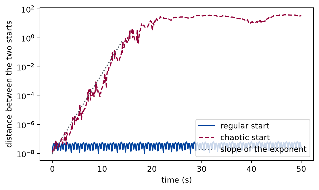— Figure 1: simulated The distance between two nearly identical starts, on a logarithmic axis. In the regular motion it grows slowly and stays far below the size of the motion; in the chaotic motion it grows along a straight line, an exponential, until it reaches the size of the motion and cannot grow any more. The dashed line has the slope of the Lyapunov exponent estimated below.

The figure is the simulation of the two starts, with the line drawn from the exponent that the next example estimates. The regular separation reaches 7e-08 at the end and the chaotic separation 40.0, which is the size of the motion itself: the starts began 1e-08 apart. The chaotic curve is straight on the logarithmic axis for the first stretch, which is what an exponential looks like, and then the separation can grow no more because the two pendulums are anywhere in the same region and the distance between two places in it is bounded.

The estimate in both regimes

def lyapunov_table(experiment: Experiment, estimates) -> list:
    """The estimate of the exponent of both starts after three lengths of
    the run; record the table and return its rows."""
    rows = []
    for name, estimate in estimates.items():
        row = [name]
        for horizon in (25.0, 50.0, 100.0):
            row.append(estimate.running[np.searchsorted(estimate.t, horizon) - 1])
        rows.append(row)

    experiment.table(
        "lyapunov-table",
        rows,
        columns=[
            ("start", "", ""),
            ("after 25 s", "1/s", ".3f"),
            ("after 50 s", "1/s", ".3f"),
            ("after 100 s", "1/s", ".3f"),
        ],
        caption="The estimate of the largest Lyapunov exponent of the two starts of "
        "the figure, after three lengths of the run, to three decimals.",
    )
    return rows

src/pbc/mechanics/experiments/double_pendulum_chaos.py, lines 175 to 197, read from the repository when this page was built.

The estimate of the largest Lyapunov exponent of the two starts of the figure, after three lengths of the run, to three decimals.
start	after 25 s (1/s)	after 50 s (1/s)	after 100 s (1/s)
regular	0.022	0.011	0.010
chaotic	1.284	1.156	1.275

Numerically verified (the two starts, one hundred seconds, classical Runge-Kutta method, separation one hundred-millionth): The estimate for the regular start falls with the length of the run and ends near zero, and the estimate for the chaotic start is positive and steady: the regular estimate went from 0.022 to 0.010 per second, the chaotic one from 1.28 to 1.27. So a lone number is not the evidence, the behaviour with the length of the run is. The chaotic value corresponds to a factor of $e$ in the separation every 0.78 s.

The estimator itself has to be checked on a case where the answer is known. A particle at a hyperbolic point, with $\ddot x = \lambda^2 x$ , has the exponent $\lambda$ exactly, and the same code estimates it:

def known_exponent(experiment: Experiment) -> None:
    """The estimator on the hyperbolic point, whose exponent is known;
    record the table."""
    known = 1.3  # 1/s
    check = lyapunov_exponent(
        State(t=0.0, x=[0.0], v=[0.0]),
        lambda t, x, v: known**2 * x,
        dt=0.01,
        n_steps=3000,
        separation=1e-6,
    )
    experiment.table(
        "known-exponent",
        [(known, check.exponent, abs(check.exponent / known - 1.0))],
        columns=[
            ("exponent", "1/s", ".3f"),
            ("estimate", "1/s", ".4f"),
            ("relative difference", "", ".1e"),
        ],
        caption="The estimator on the hyperbolic point, whose exponent is known, "
        "to the precision shown.",
    )

src/pbc/mechanics/experiments/double_pendulum_chaos.py, lines 200 to 221, read from the repository when this page was built.

The estimator on the hyperbolic point, whose exponent is known, to the precision shown.
exponent (1/s)	estimate (1/s)	relative difference
1.300	1.3009	6.6e-04

Numerically verified (the linear hyperbolic point, thirty seconds): The estimator recovers the known exponent to a fraction of a per cent; the small remainder is the first interval, before the second start has lined up with the growing direction.

What a finer step changes

A chaotic trajectory amplifies the error of every step, so a run with half the step is a different trajectory after a while. The cell compares the two trajectories of the chaotic start and the estimates of the exponent from them.

def step_halved(experiment: Experiment, chaotic_run, estimates):
    """The chaotic start at half the step: when the two runs part, and the
    estimate of the exponent; record the table."""
    fine = 0.005  # s
    coarse_run = chaotic_run
    fine_run = simulate(
        chaotic_start, pendulum, fine, round(50.0 / fine), step=rk4_step
    )
    gap = np.linalg.norm(
        np.hstack([coarse_run.x - fine_run.x[::2], coarse_run.v - fine_run.v[::2]]),
        axis=1,
    )
    diverged = coarse_run.t[np.argmax(gap > 1e-3)]
    fine_estimate = lyapunov_exponent(
        chaotic_start, pendulum, fine, round(100.0 / fine), rescale_every=20
    )

    experiment.table(
        "step-halved",
        [
            ("step of the first run", dt, estimates["chaotic"].exponent),
            ("half the step", fine, fine_estimate.exponent),
        ],
        columns=[
            ("run", "", ""),
            ("step", "s", ".3f"),
            ("estimate after 100 s", "1/s", ".3f"),
        ],
        caption="The estimate of the exponent of the chaotic start at two steps, to "
        "three decimals.",
    )
    return diverged, fine_estimate

src/pbc/mechanics/experiments/double_pendulum_chaos.py, lines 224 to 255, read from the repository when this page was built.

The estimate of the exponent of the chaotic start at two steps, to three decimals.
run	step (s)	estimate after 100 s (1/s)
step of the first run	0.010	1.275
half the step	0.005	1.284

The trajectories agree until 5 s and then differ by more than a thousandth: after that time the position of the pendulum depends on the step, and no change of method restores it. The exponent is the same to within 1%, because it is a property of the motion as a whole that the step does not change. This is what a chaotic simulation can claim: the first seconds as a trajectory, and the exponent as a statistic.

Limits

The double pendulum is one system at one energy. The exponent of a start depends on where it begins, as the first exercise shows: the motion changes from regular to chaotic with the energy, and there is no single exponent for the pendulum.
The estimate is finite-time and finite-separation. For the chaotic start the estimate settles to a few per cent between runs of different length and between steps, not to the digits shown, and no confidence interval is computed here.
The estimator follows one direction of the separation, the largest. A system has one exponent per direction, and their sum says how a volume of starts contracts or expands; the lesson on phase space returns to it.
A Lyapunov exponent is not proof of chaos. A positive finite-time estimate can come from an unstable motion that leaves for infinity, or from a rescaling too coarse for the motion; the check here is that the estimate is positive, steady with the length of the run, and absent in the regular start.
The accuracy of a single chaotic trajectory is not claimed beyond the time after which the finer step disagrees with the coarser one.
The equations are checked through the linear modes and the energy. A mistake in a nonlinear term that leaves both unchanged would pass; the next lesson compares the equations with an independent derivation.

Self-check. A colleague reports a positive Lyapunov estimate of one per second for a pendulum and says that the simulated trajectory of one minute is therefore unreliable and the whole simulation is worthless. What do you answer, and what would you compute to find out what the simulation can be used for?

With scripts, you can record in this browser that you answered this question.

Solution to the self-check

The sign says that errors grow exponentially, not that the simulation is wrong. An error is multiplied by a factor of $e$ every second, so the trajectory is reliable for the horizon $t_h \approx \ln(\Delta/d_0)$ seconds, the logarithm of the tolerated error over the error of the start, and unreliable beyond it. The simulation is still good for what does not depend on the single path: the exponent itself, the energy, the region the motion fills. To find out, repeat the run with a finer step, as the last worked example does, and take the time at which the two runs part as the horizon of this simulation; check the energy drift. A trajectory-by-trajectory use needs the horizon, a statistical use does not.

Exercises

Exercise 1. How long can it be predicted? The start of the chaotic pendulum is known to one millionth of a radian. Using the exponent of the chaotic start, estimate how long a prediction stays within a phase-space distance of a hundredth (radians and radians per second, equal weight) of the true motion, then measure it by a simulation of the start and of the start moved by the error.

Hint 1 of 2 for exercise 1

The horizon is the logarithm of the tolerated error over the error of the start, divided by the exponent.

Hint 2 of 2 for exercise 1

Measure the time at which the distance between the runs first exceeds the tolerance, and expect it to be of the order of the formula, not equal to it.

Solution to exercise 1

def prediction_horizon(experiment: Experiment, chaotic_run, rate):
    """Exercise 1: the time to lose a distance of a hundredth from a start
    known to a millionth, from the exponent and measured; record the
    table."""
    d0, tolerance = 1e-6, 1e-2
    horizon = np.log(tolerance / d0) / rate
    other = run_for(
        State(0.0, chaotic_start.x + np.array([d0, 0.0]), chaotic_start.v), 50.0
    )
    gap_curve = separation(chaotic_run, other)
    measured = chaotic_run.t[np.argmax(gap_curve > tolerance)]

    experiment.table(
        "prediction-horizon",
        [(horizon, measured)],
        columns=[("from the exponent", "s", ".1f"), ("measured", "s", ".1f")],
        caption="The time to lose a phase-space distance of a hundredth from a "
        "start known to a millionth of a radian, to one decimal.",
    )
    return horizon, measured

src/pbc/mechanics/experiments/double_pendulum_chaos.py, lines 258 to 277, read from the repository when this page was built.

The time to lose a phase-space distance of a hundredth from a start known to a millionth of a radian, to one decimal.
from the exponent (s)	measured (s)
7.2	7.1

The two agree to the factor that the fluctuation of the growth rate along the path allows, 0.98. A hundred times better knowledge of the start, an error of $d_0/100$ , adds 3.6 s: the logarithm that the formula promises.

Exercise 2. Where does the chaos begin? Release the pendulum at rest with both rods at the same angle, for the angles 0.5, 1.0, 1.5, 2.0, and 2.5 radians, and estimate the exponent over fifty seconds for each. At which of these angles does the sign of the behaviour change?

Hint 1 of 1 for exercise 2

Read each estimate at twenty-five and at fifty seconds. A regular start has an estimate that falls; a chaotic one holds.

Solution to exercise 2

def energy_scan(experiment: Experiment) -> list:
    """Exercise 2: the estimate of the exponent for five starts of increasing
    energy; record the table and return its rows."""
    rows = []
    for angle in (0.5, 1.0, 1.5, 2.0, 2.5):
        estimate = lyapunov_exponent(
            released(angle, angle), pendulum, dt, round(50.0 / dt)
        )
        middle = estimate.running[np.searchsorted(estimate.t, 25.0) - 1]
        rows.append((angle, middle, estimate.exponent))

    experiment.table(
        "energy-scan",
        rows,
        columns=[
            ("both angles", "rad", ".1f"),
            ("estimate after 25 s", "1/s", ".3f"),
            ("estimate after 50 s", "1/s", ".3f"),
        ],
        caption="The estimate of the exponent for five starts of increasing "
        "energy, to three decimals.",
    )
    return rows

src/pbc/mechanics/experiments/double_pendulum_chaos.py, lines 280 to 302, read from the repository when this page was built.

The estimate of the exponent for five starts of increasing energy, to three decimals.
both angles (rad)	estimate after 25 s (1/s)	estimate after 50 s (1/s)
0.5	0.056	0.032
1.0	0.091	0.059
1.5	0.764	0.720
2.0	1.284	1.156
2.5	1.891	1.448

The estimate falls between twenty-five and fifty seconds by 43% and 35% at the two smallest angles, and is a factor of 8 larger, and nearly steady (6% change), at 1.5 rad. Within these five starts the change from regular to chaotic is between the second and the third. The line is not sharp: the double pendulum has regular and chaotic starts at the same energy near the transition, a single estimate of fifty seconds can mistake a long regular episode for chaos, and a single pair of angles does not draw the boundary.

Run this experiment

This page was built from commit 6417e2ff90258bd2d2ba21d217eb7666fd24f680 of the repository.

In a clone at that commit, with the project’s Python packages installed, this command runs the experiment of this page:

uv run --locked --no-dev python -m pbc.mechanics.experiments.double_pendulum_chaos results

Files, tests, and every command

The files behind it:

site/lessons/mechanics/13-double-pendulum-chaos/index.qmd: this page, with every code cell.
src/pbc/mechanics/dynamics.py: code the experiment runs.
src/pbc/mechanics/integrators.py: code the experiment runs.
src/pbc/mechanics/chaos.py: code the experiment runs.
src/pbc/mechanics/experiments/double_pendulum_chaos.py: code the experiment runs.
src/pbc/experiment.py: code the experiment runs.
tests/unit/test_dynamics.py: tests of that code.
tests/unit/test_integrators.py: tests of that code.
tests/unit/test_chaos.py: tests of that code.
tests/unit/test_double_pendulum_chaos_experiment.py: tests of that code.

With Git and uv installed (see the setup page), run:

git clone https://github.com/taspinar/physics-by-construction.git
cd physics-by-construction
git checkout 6417e2ff90258bd2d2ba21d217eb7666fd24f680
uv sync --locked --no-dev
uv run --locked --no-dev python -m pbc.mechanics.experiments.double_pendulum_chaos results

The experiment writes every figure of this page into results/, as <label>.png, and every number and table of the page, as the page shows it, into results/results.json. Its numbers match this page to the digits shown, and its figure files are the ones the page shows; digits beyond those can differ between machines, because floating-point libraries differ. Change the code of the experiment and run it again to see what changes.