Lagrangian mechanics

The equations of motion of a constrained or coupled system from one function, the kinetic minus the potential energy, simulated and checked against the Newtonian form for the pendulum, two coupled springs, a planet, and the equations of the double pendulum.

Course

Classical mechanics, lesson 10 of 28

Slot

M10, Lagrangian mechanics

Methods

Simulation

Difficulty

Advanced, level 3 of 3

What you’ll learn

Write the Lagrangian of a system in coordinates that fit its constraints
Obtain and simulate its equations of motion from the Euler-Lagrange equations
Check the equations against the Newtonian form in cases with a closed form
Read a conserved momentum off a coordinate that the Lagrangian does not contain

Prerequisites

Energy conservation, Double pendulum and chaos.

Before you begin

Calculus: partial derivatives, and the chain rule for a function of several variables
Linear algebra: solving a system of linear equations written with a matrix
Trigonometry: the sine and cosine, and polar coordinates

Related

Hamiltonian mechanics

Previous

Double pendulum and chaos

Next

Hamiltonian mechanics

With scripts, this page keeps a record in your browser of whether you completed the lesson. Nothing is stored without them.

With scripts, this place suggests what to do next, with the reason, from the progress saved in your browser. Without them, follow the learning path.

A bead slides on a wire bent into a curve, a bob swings on a rod, two masses are tied by springs. Newton’s second law applies to every one of them, but in the form of the first lesson it needs the forces, and some of those are forces nobody chooses: the push of the wire on the bead, the tension in the rod. They are whatever it takes to keep the motion on the curve, and they depend on the motion. The pendulum of the energy lesson avoided them by resolving the weight along the arc and keeping one coordinate. Doing that for a rod with a second rod hung from it, as the previous lesson did and only stated the result, is a page of geometry, and a slip in it is not visible.

This lesson replaces the geometry with a procedure. Write down the kinetic and the potential energy in whatever coordinates fit the system, form their difference, and take derivatives. The result is the equations of motion, with no force of constraint in them, and the program that takes the derivatives is short enough to check on cases where Newton’s law can be solved. The lesson checks it on the pendulum, on two coupled springs, on a planet in polar coordinates, and on the double pendulum of the previous lesson, whose equations it thereby compares with an independent derivation.

Assumptions

The model and the program rest on these assumptions. Each one names what goes wrong when it does not hold.

Ideal constraints. The forces that hold the system on its constraint do no work, as the tension of a rod or the push of a smooth wire does not. With friction on the wire the procedure gives the wrong motion, because the friction does work along the path and is not in the potential.
Forces from a potential. Every force that is not a constraint comes from a potential energy that depends on the coordinates. A drag, which depends on the velocity and does negative work, is not in $U$ ; it enters as a generalised force, which this lesson does not need.
Coordinates that describe the configuration completely and independently. One angle for the pendulum, two for the double pendulum. With more coordinates than degrees of freedom the equations need the constraints added, and the matrix of the next section would have no inverse.
A kinetic energy quadratic in the velocities. The program solves a linear system for the accelerations, which needs that. Relativistic motion and motion in a magnetic field have Lagrangians that are not of this form.
Derivatives by central differences. The program takes the derivatives of the Lagrangian numerically, with a step that is a compromise between truncation and round-off; its accuracy, near one part in a million, is measured below and limits every agreement the lesson reports.
The equations are as accurate as the stepper. The simulations use the classical Runge-Kutta method with a step far below the fastest time scale.

From a function to the equations of motion

The Euler-Lagrange equations

Let the configuration of a system be given by the generalised coordinates $q_1, \dots, q_n$ , and write $\dot q_i$ for their rates of change. The Lagrangian is the kinetic energy minus the potential energy, as a function of the coordinates and their rates,

$L(q, \dot q) = T(q, \dot q) - U(q),$

and the motion obeys the Euler-Lagrange equations,

$\frac{\mathrm{d}}{\mathrm{d}t}\frac{\partial L}{\partial \dot q_i} = \frac{\partial L}{\partial q_i}, \qquad i = 1, \dots, n .$

They follow from requiring that the motion makes the time integral of $L$ stationary among nearby paths with the same ends, the principle of stationary action; this lesson takes them as given and checks what they say.

For a particle on a line, $L = \tfrac12 m \dot x^2 - U(x)$ , so $\partial L/\partial \dot x = m\dot x$ , whose time derivative is $m\ddot x$ , and $\partial L/\partial x = -U'(x)$ . The equation is $m\ddot x = -U'(x)$ , Newton’s second law with the force minus the gradient of the potential. In Cartesian coordinates the new procedure is the old law, written differently. The gain is that nothing in the equations depends on the coordinates being Cartesian.

A pendulum, a constraint that is not there

The bob of a pendulum on a rod of length $l$ is at the position $(l\sin\theta, -l\cos\theta)$ , with $\theta$ the angle from the downward vertical, so its speed is $l\dot\theta$ and its height $-l\cos\theta$ . The Lagrangian has one coordinate,

$L = \tfrac12 m l^2 \dot\theta^2 + m g l \cos\theta,$

and the Euler-Lagrange equation reads $\mathrm{d}(m l^2\dot\theta)/\mathrm{d}t = -m g l \sin\theta$ , so

$\ddot\theta = -\frac{g}{l}\sin\theta .$

This is the equation of the energy lesson, got without resolving a force along an arc and without the tension of the rod, which has dropped out because it does no work. The tension is lost with it: the equation says nothing about it, and a design that needs the tension needs Newton’s law in the plane.

Coupled coordinates

Two equal masses sit between two walls, each held to its wall by a spring $k$ and to each other by a spring $\kappa$ . With the displacements $x_1$ and $x_2$ from rest,

$L = \tfrac12 m(\dot x_1^2 + \dot x_2^2) - \tfrac12 k (x_1^2 + x_2^2) - \tfrac12 \kappa (x_1 - x_2)^2 .$

The equations are $m\ddot x_1 = -k x_1 - \kappa(x_1 - x_2)$ and the same with the indices swapped, which is what Newton’s law gives from the three spring forces. The sum and the difference of the coordinates decouple them. In phase, $x_1 = x_2$ , the middle spring is not stretched and the frequency is $\omega_+^2 = k/m$ ; out of phase, $x_1 = -x_2$ , it is stretched twice as much as either, and $\omega_-^2 = (k + 2\kappa)/m$ . These are the closed forms that the program is checked against.

The matrix form, and the double pendulum

For a kinetic energy quadratic in the rates, $T = \tfrac12 \dot q^{\mathsf T} M(q)\,\dot q$ with a symmetric mass matrix $M$ , the Euler-Lagrange equations are linear in the accelerations. Expanding the time derivative of $\partial L/\partial \dot q_i$ with the chain rule gives

$\sum_j \frac{\partial^2 L}{\partial \dot q_i\,\partial \dot q_j}\,\ddot q_j = \frac{\partial L}{\partial q_i} - \sum_j \frac{\partial^2 L}{\partial \dot q_i\,\partial q_j}\,\dot q_j ,$

and the matrix on the left is $M$ . The program forms these four arrays by central differences of $L$ and solves for $\ddot q$ . For the double pendulum the Lagrangian is written from the positions of the two bobs, with the angles as coordinates and the velocities by the chain rule, and everything else is done by the program. The equations of the previous lesson are what this gives in closed form, and the lesson compares them below.

What is conserved

If a coordinate does not appear in $L$ , its equation says $\mathrm{d}p/\mathrm{d}t = 0$ for the generalised momentum $p_i = \partial L/\partial \dot q_i$ : the momentum conjugate to a cyclic coordinate is conserved. And if $L$ does not depend on the time, the quantity $E = \sum_i p_i \dot q_i - L$ is conserved, the energy; for $L = T - U$ with $T$ quadratic in the rates it is $T + U$ . A planet in the plane of its orbit shows both. In polar coordinates $(r, \phi)$ ,

$L = \tfrac12 m(\dot r^2 + r^2\dot\phi^2) + \frac{G M m}{r},$

the angle $\phi$ is absent, so $p_\phi = m r^2\dot\phi$ , the angular momentum, is conserved: the second law of Kepler, as a consequence of the form of $L$ rather than of a calculation. The planet in these coordinates also has a closed form to check the program against, the period of a bound orbit.

The program

The reusable code is pbc.mechanics.lagrangian. A Lagrangian is a function of two vectors, the coordinates and their rates, that returns joules; the Euler-Lagrange operator turns it into an acceleration in the sense of the stepping interface, so the simulations of the earlier lessons apply.

def euler_lagrange(lagrangian: Lagrangian, h: float = DIFFERENCE_STEP) -> Acceleration:
    """The accelerations a(t, q, qdot) that the Euler-Lagrange equations of
    ``lagrangian`` give, as an acceleration for the steppers.

    ``h`` is the step of the central differences, in the units of the
    coordinates. The Lagrangian must be quadratic enough that the matrix of
    its second derivatives in the rates is invertible (the mass matrix).
    """

    def acceleration(t: float, q: Vector, qdot: Vector) -> Vector:
        force, _, mass, mixed = _derivatives(lagrangian, q, qdot, h)
        return np.linalg.solve(mass, force - mixed @ qdot)

    return acceleration

Line 100, force, _, mass, mixed = _derivatives(lagrangian, q, qdot, h): The four arrays of derivatives of the Lagrangian, by central differences with the step ``h``: the generalised forces, the momenta, the mass matrix, and the mixed second derivatives.
Line 101, return np.linalg.solve(mass, force - mixed @ qdot): The linear system of the explanation, solved for the accelerations: mass matrix times acceleration equals the force minus the mixed term times the rates.

src/pbc/mechanics/lagrangian.py, lines 90 to 103, read from the repository when this page was built.

The generalised momentum and the energy function, which the conservation laws of the explanation use:

def generalised_momentum(
    lagrangian: Lagrangian, q: Vector, qdot: Vector, h: float = DIFFERENCE_STEP
) -> Vector:
    """The momenta p = ∂L/∂q̇ conjugate to the coordinates ``q``.

    For a Cartesian coordinate it is the momentum m v; for an angle it is the
    angular momentum. A coordinate that L does not contain (a cyclic one) has
    a momentum that the motion keeps constant.
    """
    n = len(q)
    return np.array(
        [
            (
                lagrangian(q, qdot + _unit(n, i) * h)
                - lagrangian(q, qdot - _unit(n, i) * h)
            )
            / (2 * h)
            for i in range(n)
        ]
    )

src/pbc/mechanics/lagrangian.py, lines 106 to 125, read from the repository when this page was built.

def energy_function(
    lagrangian: Lagrangian, q: Vector, qdot: Vector, h: float = DIFFERENCE_STEP
) -> float:
    """The energy E = p·q̇ - L in J that a time-independent Lagrangian
    conserves; it is the kinetic plus the potential energy when L = T - U and
    T is quadratic in the rates."""
    return float(
        generalised_momentum(lagrangian, q, qdot, h) @ qdot - lagrangian(q, qdot)
    )

src/pbc/mechanics/lagrangian.py, lines 128 to 136, read from the repository when this page was built.

The three Lagrangians of the module. The last is written from the positions of the bobs and nothing else.

def pendulum_lagrangian(
    mass: float, length: float, g: float = STANDARD_GRAVITY
) -> Lagrangian:
    """The Lagrangian of a pendulum, with the angle θ from the downward
    vertical as the only coordinate: the rod's constraint is built in, and its
    tension appears nowhere."""

    def lagrangian(q: Vector, qdot: Vector) -> float:
        return float(
            0.5 * mass * length**2 * qdot[0] ** 2 + mass * g * length * np.cos(q[0])
        )

    return lagrangian

src/pbc/mechanics/lagrangian.py, lines 139 to 151, read from the repository when this page was built.

def coupled_springs_lagrangian(mass: float, k: float, coupling: float) -> Lagrangian:
    """The Lagrangian of two equal masses (kg) between two walls, each held
    by a spring ``k`` (N/m) and joined to the other by a spring ``coupling``
    (N/m); the coordinates are the two displacements from rest."""

    def lagrangian(q: Vector, qdot: Vector) -> float:
        kinetic = 0.5 * mass * float(qdot @ qdot)
        potential = 0.5 * k * float(q @ q) + 0.5 * coupling * float((q[0] - q[1]) ** 2)
        return kinetic - potential

    return lagrangian

src/pbc/mechanics/lagrangian.py, lines 154 to 164, read from the repository when this page was built.

def double_pendulum_lagrangian(
    m1: float, m2: float, l1: float, l2: float, g: float = STANDARD_GRAVITY
) -> Lagrangian:
    """The Lagrangian of the double pendulum, with the two rod angles from the
    downward vertical as coordinates.

    It is written from the Cartesian positions of the two bobs, and their
    velocities follow from the chain rule, so nothing is derived by hand.
    """

    def lagrangian(q: Vector, qdot: Vector) -> float:
        vx1 = l1 * np.cos(q[0]) * qdot[0]
        vy1 = l1 * np.sin(q[0]) * qdot[0]
        vx2 = vx1 + l2 * np.cos(q[1]) * qdot[1]
        vy2 = vy1 + l2 * np.sin(q[1]) * qdot[1]
        kinetic = 0.5 * m1 * (vx1**2 + vy1**2) + 0.5 * m2 * (vx2**2 + vy2**2)
        height1 = -l1 * np.cos(q[0])
        height2 = height1 - l2 * np.cos(q[1])
        return float(kinetic - m1 * g * height1 - m2 * g * height2)

    return lagrangian

Line 180, vx2 = vx1 + l2 * np.cos(q[1]) * qdot[1]: The velocity of the second bob is that of the first plus its own motion about it: the chain rule, not a derivation by hand.
Line 185, return float(kinetic - m1 * g * height1 - m2 * g * height2): The kinetic energy minus the potential energy, the weights times the heights below the pivot.

src/pbc/mechanics/lagrangian.py, lines 167 to 187, read from the repository when this page was built.

Worked examples

The pendulum against the Newtonian form

The pendulum is one kilogram on a one-metre rod. The Newtonian form is the tangential weight of the energy lesson. The cell compares the accelerations of the two at several angles, and then simulates the Lagrangian pendulum and compares its period with the elliptic integral.

mass, length = 1.0, 1.0
from_lagrangian = euler_lagrange(pendulum_lagrangian(mass, length))
newtonian = newton(mass, pendulum_force(mass, length))

src/pbc/mechanics/experiments/lagrangian_mechanics.py, lines 37 to 39, read from the repository when this page was built.

def pendulum_check(experiment: Experiment) -> list:
    """The acceleration of the pendulum bob along the arc at four angles,
    from Newton's law and from the Lagrangian; record the table and return
    its rows."""
    rows = []
    for angle in (0.1, 1.0, 2.0, 3.0):
        theta, rate = np.array([angle]), np.array([0.7])
        a_lagrange = length * from_lagrangian(0.0, theta, rate)[0]
        a_newton = newtonian(0.0, length * theta, rate)[0]
        rows.append((angle, a_newton, a_lagrange, abs(a_lagrange / a_newton - 1.0)))

    experiment.table(
        "pendulum-check",
        rows,
        columns=[
            ("angle", "rad", ".1f"),
            ("acceleration along the arc, Newton", "m/s²", ".5f"),
            ("from the Lagrangian", "m/s²", ".5f"),
            ("relative difference", "", ".1e"),
        ],
        caption="Acceleration of the pendulum bob along the arc at four angles, "
        "from the tangential weight and from the Euler-Lagrange equation, with "
        "the relative difference.",
    )
    return rows

src/pbc/mechanics/experiments/lagrangian_mechanics.py, lines 47 to 71, read from the repository when this page was built.

Acceleration of the pendulum bob along the arc at four angles, from the tangential weight and from the Euler-Lagrange equation, with the relative difference.
angle (rad)	acceleration along the arc, Newton (m/s²)	from the Lagrangian (m/s²)	relative difference
0.1	-0.97903	-0.97903	1.7e-07
1.0	-8.25201	-8.25201	1.7e-07
2.0	-8.91716	-8.91716	1.7e-07
3.0	-1.38391	-1.38391	1.7e-07

Numerically verified (the pendulum, four angles, any velocity because the force does not depend on it): The equation from the Lagrangian is the Newtonian one: the largest relative difference is 2e-07, which is the accuracy of the central differences. A simulation then has to reproduce a result that nothing but the exact equation gives, the period at large amplitude:

def pendulum_period_check(experiment: Experiment):
    """The period of the Lagrangian pendulum at a large amplitude, from a
    quarter swing; record the table."""
    amplitude = 1.5  # rad
    dt = 0.01  # s
    swing = simulate(
        State(0.0, [amplitude], [0.0]), from_lagrangian, dt, 400, step=rk4_step
    )
    below = np.where((swing.x[:-1, 0] > 0) & (swing.x[1:, 0] <= 0))[0][0]
    quarter = (
        swing.t[below]
        + swing.x[below, 0] / (swing.x[below, 0] - swing.x[below + 1, 0]) * dt
    )

    experiment.table(
        "pendulum-period",
        [(amplitude, pendulum_period(length, amplitude), 4 * quarter)],
        columns=[
            ("amplitude", "rad", ".1f"),
            ("period, elliptic integral", "s", ".5f"),
            ("period, simulation", "s", ".5f"),
        ],
        caption="Period of the Lagrangian pendulum at a large amplitude, from the "
        "closed form and from the simulation, to five decimals.",
    )
    return amplitude, quarter

src/pbc/mechanics/experiments/lagrangian_mechanics.py, lines 74 to 99, read from the repository when this page was built.

Period of the Lagrangian pendulum at a large amplitude, from the closed form and from the simulation, to five decimals.
amplitude (rad)	period, elliptic integral (s)	period, simulation (s)
1.5	2.33138	2.33139

Numerically verified (amplitude of one and a half radians, classical Runge-Kutta method): The simulated period of the Lagrangian pendulum is the closed-form one, to a relative 3e-07.

Two coupled springs

The masses are half a kilogram, the wall springs four newtons per metre, and the middle spring one and a half newtons per metre. The cell starts the system in each of the two modes, compares the Lagrangian accelerations with the closed-form $-\omega^2 x$ , and then simulates a general start with the Lagrangian and with Newton’s law and compares the paths.

def coupled_springs() -> float:
    """Ten seconds of the coupled springs from the Lagrangian against Newton's
    law; the largest difference of the paths, in m."""
    m_spring, k_wall, k_mid = 0.5, 4.0, 1.5
    springs = euler_lagrange(coupled_springs_lagrangian(m_spring, k_wall, k_mid))

    wall = spring(k_wall)

    def between(t, x, v):
        return k_mid * np.array([-(x[0] - x[1]), x[0] - x[1]])

    newtonian_springs = newton(m_spring, wall, between)
    start = State(0.0, [0.3, -0.1], [0.2, 0.5])
    by_lagrange = simulate(start, springs, 0.01, 1000, step=rk4_step)
    by_newton = simulate(start, newtonian_springs, 0.01, 1000, step=rk4_step)
    return np.max(np.abs(by_lagrange.x - by_newton.x))

src/pbc/mechanics/experiments/lagrangian_mechanics.py, lines 102 to 117, read from the repository when this page was built.

Numerically verified (the stated masses and springs): The Lagrangian reproduces both normal-mode frequencies and the two simulations, of the same start with the Lagrangian and with the forces, differ by at most 2e-12 m over ten seconds, which is round-off: for a Lagrangian that is quadratic in both the coordinates and the rates, the central differences have no truncation error, so the agreement here is far better than in the nonlinear examples.

A planet in polar coordinates

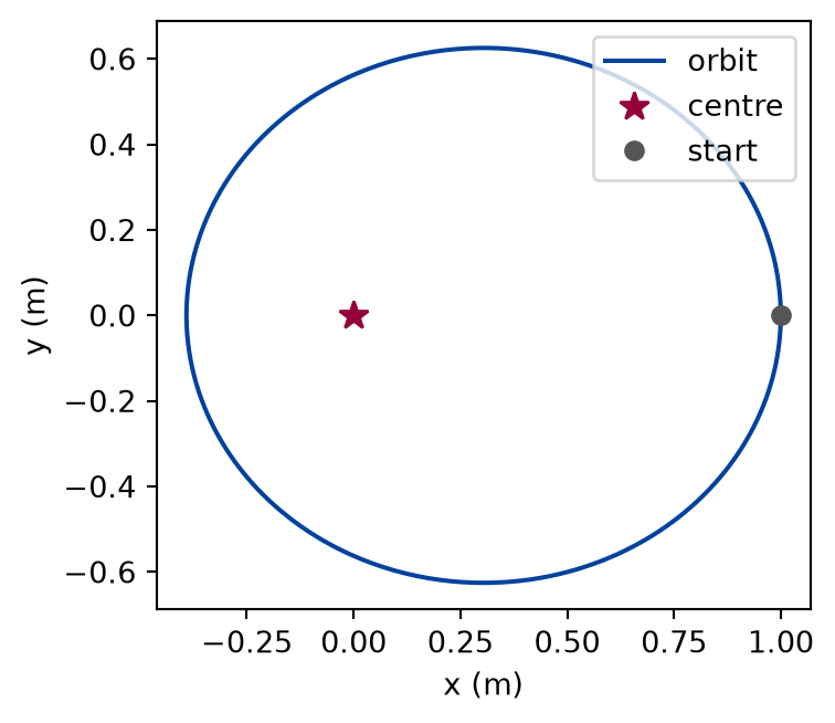
The planet has the mass one kilogram and the attraction has the strength $G M = 4\,\mathrm{m}^3/\mathrm{s}^2$ . It starts at one metre from the centre with a tangential speed of one and a half metres per second, which is below the speed of a circular orbit at that distance, so the orbit is an ellipse that starts at its far end. The cell writes the Lagrangian in $(r, \phi)$ itself, forms the equations with the Euler-Lagrange operator, and runs one period, which has a closed form from the semi-major axis $a$ , $T = 2\pi a^{3/2}/\sqrt{G M}$ , with $a$ from the energy.

def planet_lagrangian(gm, m):
    """Polar coordinates (r, phi): L = m (r'^2 + r^2 phi'^2) / 2 + G M m / r."""

    def lagrangian(q, qdot):
        return 0.5 * m * (qdot[0] ** 2 + q[0] ** 2 * qdot[1] ** 2) + gm * m / q[0]

    return lagrangian

src/pbc/mechanics/experiments/lagrangian_mechanics.py, lines 120 to 126, read from the repository when this page was built.

def planet(experiment: Experiment):
    """One orbit of a planet from its Lagrangian in polar coordinates, with
    its angular momentum and energy; record the table and return the run,
    the momenta, and the turns of the angle."""
    gm, m_planet = 4.0, 1.0
    r0, speed = 1.0, 1.5
    orbit = euler_lagrange(planet_lagrangian(gm, m_planet))
    planet_energy = 0.5 * m_planet * speed**2 - gm * m_planet / r0
    semi_major = -gm * m_planet / (2.0 * planet_energy)
    orbital_period = 2.0 * np.pi * np.sqrt(semi_major**3 / gm)

    start = State(0.0, [r0, 0.0], [0.0, speed / r0])
    steps = round(orbital_period / 0.005)
    orbit_run = simulate(start, orbit, orbital_period / steps, steps, step=rk4_step)
    lagr = planet_lagrangian(gm, m_planet)
    momentum = np.array(
        [
            generalised_momentum(lagr, x, v)[1]
            for x, v in zip(orbit_run.x, orbit_run.v, strict=True)
        ]
    )
    energies = np.array(
        [
            energy_function(lagr, x, v)
            for x, v in zip(orbit_run.x, orbit_run.v, strict=True)
        ]
    )
    turns = (orbit_run.x[-1, 1] - orbit_run.x[0, 1]) / (2 * np.pi)

    experiment.table(
        "planet",
        [
            (
                "angular momentum",
                momentum[0],
                np.max(np.abs(momentum / momentum[0] - 1.0)),
            ),
            ("energy", energies[0], np.max(np.abs(energies / energies[0] - 1.0))),
        ],
        columns=[
            ("quantity", "", ""),
            ("start", "", ".5f"),
            ("largest relative change", "", ".1e"),
        ],
        caption="Angular momentum and energy of the planet over one orbit, from "
        "the Lagrangian, at the start and the largest relative change.",
    )
    return orbit_run, momentum, turns

src/pbc/mechanics/experiments/lagrangian_mechanics.py, lines 129 to 176, read from the repository when this page was built.

Angular momentum and energy of the planet over one orbit, from the Lagrangian, at the start and the largest relative change.
quantity	start	largest relative change
angular momentum	1.50000	2.3e-08
energy	-2.87500	7.3e-06

Numerically verified (one bound orbit, classical Runge-Kutta method): The angular momentum $p_\phi$ and the energy are constant over the orbit to the accuracy of the method, as the form of $L$ says: the angular momentum is conserved because the angle is absent from it, and it changes by a relative 2e-08. The orbit is closed, as the closed form of the period says: after one period the radius is 1.00000 m, back to its start, and the angle has advanced by 1.00000 turns. The radial period of the Kepler orbit equals the angular one, which is the statement that the orbit does not precess.

def draw_planet_orbit(orbit_run) -> Figure:
    """The orbit in the plane."""
    x_plane = orbit_run.x[:, 0] * np.cos(orbit_run.x[:, 1])
    y_plane = orbit_run.x[:, 0] * np.sin(orbit_run.x[:, 1])
    fig, ax = plt.subplots(figsize=(6.4, 3.6))
    ax.plot(x_plane, y_plane, color=FIGURE_COLOURS[0], linestyle="-", label="orbit")
    ax.plot(
        [0.0],
        [0.0],
        marker="*",
        color=FIGURE_COLOURS[1],
        linestyle="",
        markersize=10,
        label="centre",
    )
    ax.plot(
        [x_plane[0]],
        [y_plane[0]],
        marker="o",
        color=FIGURE_COLOURS[2],
        linestyle="",
        label="start",
    )
    ax.set_aspect("equal")
    ax.set_xlabel("x (m)")
    ax.set_ylabel("y (m)")
    ax.legend(loc="upper right")
    return fig

src/pbc/mechanics/experiments/lagrangian_mechanics.py, lines 179 to 206, read from the repository when this page was built.

Plot of the orbit in the plane with equal axes. A closed elongated ellipse with a point marking the centre of attraction near one end of the ellipse, inside it, and a marker for the starting point at the far end of the ellipse. — Figure 1: simulated The orbit of the planet from the Euler-Lagrange equations in polar coordinates, drawn in Cartesian axes. The path closes on itself after one period, an ellipse with the attracting centre at one focus, as the period from the semi-major axis requires.

The figure is the simulation of the table, from the same run, and the closing of the curve is the check that the period of the closed form is the one that the equations give.

The equations of the double pendulum

The previous lesson gave the angular accelerations of the double pendulum in closed form. The Lagrangian here is written from the positions of the bobs, and the program takes the derivatives. The cell compares the two at random states, and then follows both from a regular start.

masses, lengths = (1.0, 2.0), (1.0, 0.7)
closed_form = double_pendulum(*masses, *lengths)

src/pbc/mechanics/experiments/lagrangian_mechanics.py, lines 42 to 43, read from the repository when this page was built.

def double_pendulum_check(experiment: Experiment) -> None:
    """The double pendulum from its Lagrangian against the closed form, at
    two hundred random states and along one regular motion; record the
    table."""
    derived = euler_lagrange(double_pendulum_lagrangian(*masses, *lengths))

    rng = np.random.default_rng(7)
    worst = 0.0
    for _ in range(200):
        q, qdot = rng.uniform(-3.0, 3.0, 2), rng.uniform(-3.0, 3.0, 2)
        a_closed, a_derived = closed_form(0.0, q, qdot), derived(0.0, q, qdot)
        worst = max(
            worst, np.max(np.abs(a_derived - a_closed) / (1.0 + np.abs(a_closed)))
        )

    regular = State(0.0, [0.3, 0.2], [0.0, 0.0])
    path_closed = simulate(regular, closed_form, 0.01, 1000, step=rk4_step)
    path_derived = simulate(regular, derived, 0.01, 1000, step=rk4_step)
    path_difference = np.max(np.abs(path_closed.x - path_derived.x))

    experiment.table(
        "double-pendulum-check",
        [(worst, path_difference)],
        columns=[
            ("largest relative difference of the accelerations", "", ".1e"),
            ("largest difference of the angles over ten seconds", "rad", ".1e"),
        ],
        caption="The equations of the double pendulum from the Lagrangian against "
        "the closed form of the previous lesson, at two hundred random states and "
        "along one regular motion.",
    )

src/pbc/mechanics/experiments/lagrangian_mechanics.py, lines 209 to 239, read from the repository when this page was built.

The equations of the double pendulum from the Lagrangian against the closed form of the previous lesson, at two hundred random states and along one regular motion.
largest relative difference of the accelerations	largest difference of the angles over ten seconds (rad)
1.6e-07	1.2e-06

Numerically verified (unequal masses and rods, two hundred random states and a regular start): The closed-form accelerations of the double pendulum agree with the Euler-Lagrange equations of its Lagrangian. That removes the caveat of the previous lesson: its equations were checked by the linear modes and the energy, and now also by an independent derivation, the nonlinear terms included. The agreement is to the accuracy of the central differences, so a mistake smaller than that would not show.

Limits

The agreement of the equations is to the accuracy of the central differences, about one part in a million at the step of the module. The last exercise measures how it depends on the step. A closed form with an error below that is not found by this check.
The derivatives are numerical, so the program is slower than the closed form (each acceleration needs dozens of evaluations of the Lagrangian) and its error is not controlled by the stepper. A symbolic derivation gives exact equations; this lesson does not use one.
Only ideal constraints and potential forces are covered. A force that depends on the velocity, or friction, needs a generalised force, and a constraint that depends on the velocity needs multipliers; neither is treated.
The Euler-Lagrange equations are taken as given from the principle of stationary action, not derived. The lesson shows that they give Newton’s law in Cartesian coordinates and agree with it in the cases checked, which is evidence of their use and not a proof of their generality.
The tension of a rod and the push of a wire are not found. A design that needs them returns to Newton’s law with the constraint.
The conserved quantities are checked on one bound orbit. That the angular momentum is conserved whenever the angle is absent is the content of the derivation above and is not tested for other systems.

Self-check. The Lagrangian method gives the equation of the pendulum without ever computing the tension in the rod. A colleague says that this means the tension plays no role in the motion. Is that right?

With scripts, you can record in this browser that you answered this question.

Solution to the self-check

No. The tension is what keeps the bob on the circle, and the method has absorbed it into the choice of the coordinate: by describing the position with the one angle the motion is already on the circle, so the force that holds it there needs no equation. The tension does no work, since it is perpendicular to the motion, which is why the energy and the Lagrangian do not need it, but it still has a value at every instant, and it is the force that a rod must withstand. To find it, return to Newton’s law in the plane, with the acceleration towards the pivot the motion gives. The method trades the force of constraint for the coordinates; it does not say the force is zero.

Exercises

Exercise 1. The Atwood machine. Two masses, three kilograms and one kilogram, hang from a rope over a light, smooth pulley. Take the position of the heavier mass below its start as the one coordinate. Write the Lagrangian, find the acceleration with the program, and compare it with the closed form $(m_1 - m_2) g/(m_1 + m_2)$ that Newton’s law gives from the tension of the rope.

Hint 1 of 1 for exercise 1

Both masses move at the same speed, and the rope length ties the position of the second to the first, so one coordinate is enough: the kinetic energy has the sum of the masses, and the potential energy the difference.

Solution to exercise 1

m_heavy, m_light = 3.0, 1.0

src/pbc/mechanics/experiments/lagrangian_mechanics.py, line 243, read from the repository when this page was built.

def atwood(q, qdot):
    return 0.5 * (m_heavy + m_light) * qdot[0] ** 2 + (m_heavy - m_light) * g * q[0]

src/pbc/mechanics/experiments/lagrangian_mechanics.py, lines 247 to 248, read from the repository when this page was built.

def atwood_machine(experiment: Experiment) -> None:
    """Exercise 1: the acceleration of the Atwood machine from Newton's law
    and from the Lagrangian; record the table."""
    a_program = euler_lagrange(atwood)(0.0, np.array([0.0]), np.array([0.0]))[0]
    a_exact = (m_heavy - m_light) / (m_heavy + m_light) * g

    experiment.table(
        "atwood",
        [(a_exact, a_program, abs(a_program / a_exact - 1.0))],
        columns=[
            ("from Newton's law", "m/s²", ".5f"),
            ("from the Lagrangian", "m/s²", ".5f"),
            ("relative difference", "", ".1e"),
        ],
        caption="Acceleration of the Atwood machine from the tension of the rope "
        "and from the Lagrangian, to five decimals.",
    )

src/pbc/mechanics/experiments/lagrangian_mechanics.py, lines 251 to 267, read from the repository when this page was built.

Acceleration of the Atwood machine from the tension of the rope and from the Lagrangian, to five decimals.
from Newton's law (m/s²)	from the Lagrangian (m/s²)	relative difference
4.90332	4.90332	0.0e+00

The two agree to the accuracy of the derivatives. The Lagrangian has no tension in it. Newton’s law needs the tension to be eliminated between the two masses, and gives it as a by-product, 14.71 N, which the Lagrangian never computes.

Exercise 2. The step of the differences. Compare the accelerations of the double pendulum of the last example with the closed form for the difference steps 0.1, 0.01, 0.001, 0.0001, and 0.00001 at the same random states. Which step is best, and why does the error rise on both sides of it?

Hint 1 of 1 for exercise 2

There are two errors: one that falls with the step, from replacing a derivative by a difference, and one that rises as the step falls, from subtracting nearly equal numbers.

Solution to exercise 2

def difference_steps(experiment: Experiment) -> list:
    """Exercise 2: the accelerations of the double pendulum for five
    difference steps against the closed form; record the table and return
    its rows."""
    rows = []
    for h in (1e-1, 1e-2, 1e-3, 1e-4, 1e-5):
        candidate = euler_lagrange(double_pendulum_lagrangian(*masses, *lengths), h=h)
        rng = np.random.default_rng(7)
        worst_h = 0.0
        for _ in range(50):
            q, qdot = rng.uniform(-3.0, 3.0, 2), rng.uniform(-3.0, 3.0, 2)
            a_closed = closed_form(0.0, q, qdot)
            worst_h = max(
                worst_h,
                np.max(
                    np.abs(candidate(0.0, q, qdot) - a_closed)
                    / (1.0 + np.abs(a_closed))
                ),
            )
        rows.append((h, worst_h))

    experiment.table(
        "difference-steps",
        rows,
        columns=[
            ("difference step", "rad", ".0e"),
            ("largest relative difference", "", ".1e"),
        ],
        caption="Largest relative difference between the accelerations from the "
        "Lagrangian and the closed form, for five difference steps.",
    )
    return rows

src/pbc/mechanics/experiments/lagrangian_mechanics.py, lines 270 to 301, read from the repository when this page was built.

Largest relative difference between the accelerations from the Lagrangian and the closed form, for five difference steps.
difference step (rad)	largest relative difference
1e-01	1.6e-03
1e-02	1.6e-05
1e-03	1.6e-07
1e-04	1.1e-06
1e-05	1.4e-04

The error falls with the step, as the square of it, down to a step of about 1e-03, and then rises again. The first part is the truncation of the second difference. The second is round-off: a second difference divides a small difference of values of order one by the square of the step, so the error of a double-precision number is multiplied by the inverse square of the step. The best step is where the two are equal, which is why the module uses it and why a smaller step would not be better.

Run this experiment

This page was built from commit 6417e2ff90258bd2d2ba21d217eb7666fd24f680 of the repository.

In a clone at that commit, with the project’s Python packages installed, this command runs the experiment of this page:

uv run --locked --no-dev python -m pbc.mechanics.experiments.lagrangian_mechanics results

Files, tests, and every command

The files behind it:

site/lessons/mechanics/14-lagrangian-mechanics/index.qmd: this page, with every code cell.
src/pbc/mechanics/dynamics.py: code the experiment runs.
src/pbc/mechanics/integrators.py: code the experiment runs.
src/pbc/mechanics/lagrangian.py: code the experiment runs.
src/pbc/mechanics/chaos.py: code the experiment runs.
src/pbc/mechanics/pendulum.py: code the experiment runs.
src/pbc/mechanics/oscillator.py: code the experiment runs.
src/pbc/mechanics/experiments/lagrangian_mechanics.py: code the experiment runs.
src/pbc/experiment.py: code the experiment runs.
tests/unit/test_lagrangian.py: tests of that code.
tests/unit/test_chaos.py: tests of that code.
tests/unit/test_pendulum.py: tests of that code.
tests/unit/test_oscillator.py: tests of that code.
tests/unit/test_lagrangian_mechanics_experiment.py: tests of that code.

With Git and uv installed (see the setup page), run:

git clone https://github.com/taspinar/physics-by-construction.git
cd physics-by-construction
git checkout 6417e2ff90258bd2d2ba21d217eb7666fd24f680
uv sync --locked --no-dev
uv run --locked --no-dev python -m pbc.mechanics.experiments.lagrangian_mechanics results

The experiment writes every figure of this page into results/, as <label>.png, and every number and table of the page, as the page shows it, into results/results.json. Its numbers match this page to the digits shown, and its figure files are the ones the page shows; digits beyond those can differ between machines, because floating-point libraries differ. Change the code of the experiment and run it again to see what changes.