Hamiltonian mechanics

Phase space, Hamilton’s equations from the Lagrangian, the area that a symplectic step preserves and the others do not, and the modified energy that such a step conserves, checked against the conserved quantities of the numerical-integrators lesson and of the Lean lesson on symplectic Euler.

Course

Classical mechanics, lesson 11 of 28

Slot

M11, Hamiltonian mechanics

Methods

Simulation

Difficulty

Advanced, level 3 of 3

What you’ll learn

Obtain the Hamiltonian from a Lagrangian and write the motion as a flow in phase space
Measure how a step of an integrator changes the area of a region of phase space
Check that a symplectic method conserves its modified energy, on the oscillator and on the pendulum
Choose between a symplectic and a higher-order method for a given length of run

Prerequisites

Lagrangian mechanics, Numerical integrators, What symplectic Euler conserves.

Before you begin

Calculus: partial derivatives
Linear algebra: the determinant of a two-by-two matrix, and the matrix of derivatives of a map
Geometry: the area of a region bounded by a closed curve

Related

none

Previous

Lagrangian mechanics

Next

Resonance and driven oscillators

With scripts, this page keeps a record in your browser of whether you completed the lesson. Nothing is stored without them.

With scripts, this place suggests what to do next, with the reason, from the progress saved in your browser. Without them, follow the learning path.

A simulation of the Solar System runs for millions of years, and a simulation of a pendulum for a few thousand swings, and the question is the same: does the energy stay where it should? The numerical-integrators lesson found that two methods of the same order differ in this, one losing or gaining energy without end and one keeping it inside a band. The Lean lesson on symplectic Euler proved why for the harmonic oscillator, with a quantity that each step leaves exactly unchanged. Both were about one force, a spring, where the algebra closes. This lesson asks what is behind the property in general.

The answer is a geometric one. Describe the state not by the position and the velocity but by the position and the momentum, so that the motion is a flow of points in a plane. The flow of a mechanical system preserves area, and a symplectic step preserves area too. A map that preserves area cannot spiral inwards or outwards, and that is what stops the energy from running away. The lesson derives the flow from the Lagrangian of the previous lesson, measures the area that each method keeps or changes, and checks the conserved quantity of the earlier lessons on the oscillator and on the pendulum, where it is no longer exact.

Assumptions

The model and the program rest on these assumptions. Each one names what goes wrong when it does not hold.

A Lagrangian that is quadratic in the rates. The Legendre transform of the program solves a linear system for the rates in terms of the momenta, as in the previous lesson. For a Lagrangian of another form the transform is not unique, or not defined.
One degree of freedom for the area. The area of a region of the plane is the measure used. With several degrees of freedom the symplectic condition is stronger than the preservation of the volume of phase space, and the lesson does not state it.
No dissipation and no explicit time dependence. The flow preserves area and the energy. With drag the area shrinks, which is the point of drag, and with a driving force the energy changes with the time.
A small step and a smooth potential. The modified energy is the first term of an expansion in the step. It describes the numerical motion well when the step is small against the time scale of the motion, and it is not expected to hold near a step at which the method is unstable.
The step map is differentiated numerically. The Jacobian of a step is found by central differences of the stepper; its error is far below the differences reported.
Real runs have round-off. The conservation that is “exact” holds in exact arithmetic, and in a run it holds to the round-off of every step.

Phase space and the symplectic step

The Hamiltonian and its equations

The Lagrangian $L(q, \dot q)$ of the previous lesson gives the momentum $p = \partial L/\partial\dot q$ conjugate to each coordinate. The Hamiltonian is the energy written in terms of the coordinates and the momenta instead of the rates,

$H(q, p) = p\,\dot q - L,$

with $\dot q$ eliminated by solving $p = \partial L/\partial\dot q$ for it. For a particle with $L = \tfrac12 m\dot q^2 - U(q)$ the momentum is $p = m\dot q$ and $H = p^2/(2m) + U(q)$ , the kinetic energy written with the momentum plus the potential energy. The pendulum with the angle as coordinate has $p = m l^2 \dot\theta$ , the angular momentum, and $H = p^2/(2 m l^2) - m g l \cos\theta$ .

The Euler-Lagrange equations become Hamilton’s equations,

$\dot q = \frac{\partial H}{\partial p}, \qquad \dot p = -\frac{\partial H}{\partial q},$

a pair of first-order equations whose state $(q, p)$ is a point of the phase space. For one degree of freedom this is a plane, and every motion is a curve in it: the curves of the oscillator are the ellipses of the earlier lessons, and the curves of the pendulum are closed loops for swinging and open lines for going over the top.

The flow preserves area

The motion moves every point of phase space with the velocity $(\partial H/\partial p, -\partial H/\partial q)$ . The divergence of this velocity field is

$\frac{\partial}{\partial q}\frac{\partial H}{\partial p} + \frac{\partial}{\partial p}\Bigl(-\frac{\partial H}{\partial q}\Bigr) = \frac{\partial^2 H}{\partial q\,\partial p} - \frac{\partial^2 H}{\partial p\,\partial q} = 0 .$

A flow without divergence moves a region of phase space without changing its area: Liouville’s theorem. A blob of starting states is carried along, stretched into a long filament if the motion shears it, with the same area. The area is the product of the uncertainty in the position and in the momentum, so the flow cannot reduce both, and the oscillator’s ellipse is a curve that the area of the blob cannot leave.

Which steps preserve area

A step of an integrator is a map from the state at one time to the state a step later. Its Jacobian matrix $J$ holds the derivatives of the new state with respect to the old one, and the area of a small region is multiplied by the determinant of $J$ . A step whose determinant is one for every state and every step length is area-preserving, which for one degree of freedom is what symplectic means.

Write the symplectic Euler step with a unit mass and the acceleration $a(x)$ as $v' = v + a(x)\,\Delta t$ followed by $x' = x + v'\,\Delta t$ . Each half is a shear: the first changes $v$ by an amount that depends on $x$ alone, the second changes $x$ by an amount that depends on $v'$ alone. The Jacobian of a shear is a triangular matrix with ones on the diagonal, and its determinant is one for any $a$ and any step. The composition of two shears has determinant one: the step is area-preserving for every force and every step length. Velocity Verlet is a composition of three shears (half a kick, a drift, half a kick) and so is symplectic too.

Explicit Euler is $x' = x + v\,\Delta t$ and $v' = v + a(x)\,\Delta t$ together, a different map, with the Jacobian $\begin{pmatrix}1 & \Delta t\\ a'\,\Delta t & 1\end{pmatrix}$ and the determinant $1 - a'(x)\,\Delta t^2$ . With the force $-U'$ and $a' = -U''$ for a unit mass this is $1 + U''\,\Delta t^2$ , larger than one wherever the potential curves upwards. Every step of explicit Euler on a pendulum below the horizontal expands the area of phase space, which is the same fact as the growth of the energy that the earlier lessons found. The classical Runge-Kutta method has a determinant that differs from one by a high power of the step, and no step length makes it exactly one.

The modified energy

An area-preserving numerical map is the exact time- $\Delta t$ flow of a slightly different Hamiltonian system, in the sense of an expansion in the step: $\tilde H = H + \Delta t\,H_1 + \Delta t^2 H_2 + \dots$ , a series that need not converge but that, cut after a few terms, describes the numerical motion to a high order for a long time. The numerical motion conserves $\tilde H$ and therefore keeps the true energy $H$ within the difference $\tilde H - H$ , which is small, of the order of the step, and does not grow.

For symplectic Euler as written, the first term is $H_1 = -\tfrac12\,\dfrac{\partial H}{\partial q}\dfrac{\partial H}{\partial p}$ , so for $H = p^2/2m + U(q)$ with $p/m = v$

$\tilde E = E - \tfrac12\,\Delta t\;U'(x)\,v .$

For the oscillator, $U' = k x$ and this is the quantity of the Lean lesson, which is conserved exactly; the series stops after the first term. For another potential it is conserved up to terms of second order in the step. For velocity Verlet the first correction is of order $\Delta t^2$ , and on the oscillator it is the closed form of the numerical-integrators lesson. The next sections check all of this by running.

The program

The code is pbc.mechanics.hamiltonian. The Legendre transform takes a Lagrangian of the previous lesson and returns the Hamiltonian; the other functions measure the area-preservation of a step and the modified energies.

def legendre_hamiltonian(
    lagrangian: Lagrangian, h: float = DIFFERENCE_STEP
) -> Hamiltonian:
    """The Hamiltonian H(q, p) = p·q̇ - L of a ``lagrangian`` that is
    quadratic in the rates q̇ (as T - U is), by the Legendre transform.

    The momentum is p = W q̇ + p₀ with the mass matrix W and the momentum p₀
    at q̇ = 0 (zero for L = T - U); the transform solves it for q̇.
    """

    def hamiltonian(q: Vector, p: Vector) -> float:
        zero = np.zeros_like(q)
        _, _, mass, _ = _derivatives(lagrangian, q, zero, h)
        p0 = generalised_momentum(lagrangian, q, zero, h)
        qdot = np.linalg.solve(mass, p - p0)
        return float(p @ qdot - lagrangian(q, qdot))

    return hamiltonian

Line 50, qdot = np.linalg.solve(mass, p - p0): The rates that give the momentum, from the linear relation of the momentum to the rates: the elimination of the explanation.
Line 51, return float(p @ qdot - lagrangian(q, qdot)): The energy as the momentum times the rate minus the Lagrangian, in joules, as a function of the coordinates and the momenta.

src/pbc/mechanics/hamiltonian.py, lines 36 to 53, read from the repository when this page was built.

The Jacobian of one step, whose determinant is the factor of area:

def step_jacobian(
    step: Stepper,
    state: State,
    acceleration: Acceleration,
    dt: float,
    h: float = 1e-6,
) -> NDArray[np.float64]:
    """The Jacobian matrix of one step of ``step`` of length ``dt`` (s), as a
    map from (x, v) at the start to (x, v) at the end, by central differences
    of size ``h`` at ``state``.

    Its determinant is the factor by which the step scales the area of a
    small region of phase space: one for the exact flow of a Hamiltonian
    system and for a symplectic method, and not one for the others.
    """
    n = len(state.x)
    z = np.concatenate([state.x, state.v])

    def advance(vector: Vector) -> Vector:
        end = step(State(state.t, vector[:n], vector[n:]), acceleration, dt)
        return np.concatenate([end.x, end.v])

    jacobian = np.empty((2 * n, 2 * n))
    for j in range(2 * n):
        e = np.zeros(2 * n)
        e[j] = h
        jacobian[:, j] = (advance(z + e) - advance(z - e)) / (2 * h)
    return jacobian

Line 83, return jacobian: The matrix of derivatives of the end state with respect to the start, with the positions first and the velocities second.

src/pbc/mechanics/hamiltonian.py, lines 56 to 83, read from the repository when this page was built.

def loop_area(x: NDArray[np.float64], v: NDArray[np.float64]) -> float:
    """The area enclosed by the closed polygon through the points (x, v), by
    the shoelace formula, as a positive number. One degree of freedom."""
    return float(0.5 * abs(np.dot(x, np.roll(v, -1)) - np.dot(v, np.roll(x, -1))))

src/pbc/mechanics/hamiltonian.py, lines 86 to 89, read from the repository when this page was built.

The two modified energies. The first is general, the second the closed form of the numerical-integrators lesson for the oscillator.

def symplectic_euler_modified_energy(
    trajectory: Trajectory,
    mass: float,
    potential: Potential,
    gradient: Callable[[Vector], Vector],
    dt: float,
) -> NDArray[np.float64]:
    """The modified energy of symplectic Euler, in J, to first order in the
    step ``dt`` (s): E - (dt / 2) ∇U(x)·v at every instant of ``trajectory``.

    ``gradient`` is ∇U, the gradient of the ``potential`` in N. For the
    harmonic oscillator this is the quantity of lesson L3 and is conserved to
    round-off; for any other potential it is conserved up to terms of second
    order in the step.
    """
    cross = np.array(
        [gradient(x) @ v for x, v in zip(trajectory.x, trajectory.v, strict=True)]
    )
    return mechanical_energy(trajectory, mass, potential) - 0.5 * dt * cross

Line 110, return mechanical_energy(trajectory, mass, potential) - 0.5 * dt * cross: The energy minus half the step times the force term U' v of the explanation, in joules, at every instant of the run.

src/pbc/mechanics/hamiltonian.py, lines 92 to 110, read from the repository when this page was built.

def verlet_oscillator_modified_energy(
    trajectory: Trajectory, mass: float, k: float, dt: float
) -> NDArray[np.float64]:
    """The modified energy of velocity Verlet on the harmonic oscillator, in
    J: ½ m (v² + ω² (1 - ω² dt² / 4) x²), conserved to round-off (lesson M5)."""
    omega2 = k / mass
    x, v = trajectory.x[:, 0], trajectory.v[:, 0]
    return 0.5 * mass * (v**2 + omega2 * (1.0 - omega2 * dt**2 / 4.0) * x**2)

src/pbc/mechanics/hamiltonian.py, lines 113 to 120, read from the repository when this page was built.

Worked examples

From the Lagrangian to the Hamiltonian

The cell takes the Lagrangian of the pendulum and of two coupled springs from the previous lesson, transforms them by the program, and compares the result with the energy written in the momenta.

def legendre() -> float:
    """The Hamiltonian of the pendulum and of the coupled springs, written in
    the momenta and from the Legendre transform; the bound the two agree
    within, in J."""
    rows = []
    pendulum_h = legendre_hamiltonian(pendulum_lagrangian(1.0, 1.0))
    for angle, momentum in ((0.5, 1.0), (1.5, -0.8), (2.5, 2.0)):
        from_program = pendulum_h(np.array([angle]), np.array([momentum]))
        closed = 0.5 * momentum**2 - g * np.cos(angle)
        rows.append(("pendulum", angle, momentum, closed, from_program))

    springs_h = legendre_hamiltonian(coupled_springs_lagrangian(0.5, 4.0, 1.5))
    q, p = np.array([0.3, -0.2]), np.array([0.4, 0.1])
    closed = p @ p / (2 * 0.5) + 0.5 * 4.0 * q @ q + 0.5 * 1.5 * (q[0] - q[1]) ** 2
    rows.append(("two springs", q[0], p[0], closed, springs_h(q, p)))

    bound = 1e-12  # J, far above round-off for numbers of this size
    assert max(abs(r[3] - r[4]) for r in rows) < bound
    return bound

src/pbc/mechanics/experiments/hamiltonian_mechanics.py, lines 58 to 76, read from the repository when this page was built.

Numerically verified (the pendulum at three points and the coupled springs at one): The Legendre transform of the program reproduces the energy written in the momenta: the largest difference is below 1e-12 J, the bound the cell asserts.

The area of one step

The cell takes the Jacobian of one step of each method at a point of the pendulum’s motion, for a step of a tenth and of half a second, and reports its determinant. The explicit Euler value is the $1 + U''\Delta t^2$ of the explanation, checked at the same point.

pendulum = newton(1.0, pendulum_force(1.0, 1.0))
t0 = small_angle_period(1.0)

src/pbc/mechanics/experiments/hamiltonian_mechanics.py, lines 46 to 47, read from the repository when this page was built.

def shown(value):
    """A deviation at the level of the numerical derivative is shown as a
    bound."""
    return f"{value:.1e}" if abs(value) > FLOOR else "below 1e-8"

src/pbc/mechanics/experiments/hamiltonian_mechanics.py, lines 82 to 85, read from the repository when this page was built.

def determinants(experiment: Experiment):
    """The determinant of the Jacobian of one step, minus one, for four
    methods at two steps, and the formula for explicit Euler; record the
    table."""
    point = State(0.0, [1.1], [0.4])
    curvature = g * np.cos(1.1)  # U'' for the unit pendulum
    steps = (0.1, 0.5)  # s
    deviations = {}
    for name, step in METHODS:
        deviations[name] = [
            np.linalg.det(step_jacobian(step, point, pendulum, dt)) - 1.0
            for dt in steps
        ]
    euler_formula = [curvature * dt**2 for dt in steps]

    experiment.table(
        "determinants",
        [(name, *(shown(d) for d in values)) for name, values in deviations.items()],
        columns=[
            ("method", "", ""),
            ("determinant minus one, step 0.1 s", "", ""),
            ("determinant minus one, step 0.5 s", "", ""),
        ],
        caption="The determinant of the Jacobian of one step, minus one, for four "
        "methods on the pendulum at an angle of one and a tenth radians and a "
        "velocity of four tenths, at two step lengths; a deviation at the level "
        "of the numerical derivative is shown as a bound.",
    )
    return deviations, euler_formula

src/pbc/mechanics/experiments/hamiltonian_mechanics.py, lines 88 to 116, read from the repository when this page was built.

The determinant of the Jacobian of one step, minus one, for four methods on the pendulum at an angle of one and a tenth radians and a velocity of four tenths, at two step lengths; a deviation at the level of the numerical derivative is shown as a bound.
method	determinant minus one, step 0.1 s	determinant minus one, step 0.5 s
explicit Euler	4.4e-02	1.1e+00
symplectic Euler	below 1e-8	below 1e-8
velocity Verlet	below 1e-8	below 1e-8
classical Runge-Kutta	2.3e-08	-1.1e-02

Numerically verified (the pendulum at one state, two step lengths): The determinants of symplectic Euler and velocity Verlet are one for both steps, to the accuracy of the derivative, and the determinant of explicit Euler minus one is 4.45e-02 and 1.11e+00, against 4.45e-02 and 1.11e+00 from $U''\Delta t^2$ : the formula is exact for this map, as its Jacobian is the matrix of the explanation. The classical Runge-Kutta determinant differs from one by 1e-02 at the long step, orders below the first-order method, and is not exactly one for any step.

A blob of starting states

The determinants are for one step at one point. The cell follows a circle of starting states of radius a tenth around the point $(1.2\ \mathrm{rad}, 0)$ of the pendulum for two small-angle periods with each method at fifty steps per period, and compares the area enclosed by the images of the points with the starting area.

def blob(experiment: Experiment):
    """A circle of starting states after two small-angle periods with each
    method, and the area it encloses; record the table and return the
    starting circle, its images, and the rows."""
    angles = np.linspace(0.0, 2.0 * np.pi, 120, endpoint=False)
    x_start, v_start = 1.2 + 0.1 * np.cos(angles), 0.1 * np.sin(angles)
    area_start = loop_area(x_start, v_start)

    images, rows = {}, []
    for name, step in METHODS:
        ends = [
            simulate(State(0.0, [a], [b]), pendulum, t0 / 50, 100, step=step)
            for a, b in zip(x_start, v_start, strict=True)
        ]
        x_end = np.array([e.x[-1, 0] for e in ends])
        v_end = np.array([e.v[-1, 0] for e in ends])
        images[name] = (x_end, v_end)
        rows.append((name, loop_area(x_end, v_end) / area_start))

    experiment.table(
        "blob",
        rows,
        columns=[
            ("method", "", ""),
            ("area after two periods / starting area", "", ".5f"),
        ],
        caption="The area enclosed by the images of a circle of starting states "
        "of the pendulum after two small-angle periods, relative to the starting "
        "area, to five decimals.",
    )
    return x_start, v_start, images, rows

src/pbc/mechanics/experiments/hamiltonian_mechanics.py, lines 119 to 149, read from the repository when this page was built.

The area enclosed by the images of a circle of starting states of the pendulum after two small-angle periods, relative to the starting area, to five decimals.
method	area after two periods / starting area
explicit Euler	1.66658
symplectic Euler	0.99997
velocity Verlet	0.99997
classical Runge-Kutta	0.99996

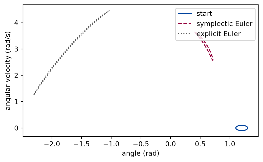
Numerically verified (one circle of starts, two small-angle periods, fifty steps per period): The two symplectic methods keep the area to the accuracy of the polygon of the images, and explicit Euler enlarges it: the area has been multiplied by 1.67 for explicit Euler and by 1.0000 and 1.0000 for the two symplectic methods. The Runge-Kutta area is within 4e-05 of the start, which this measurement cannot tell from one, because the polygon of a hundred and twenty points has an error of about that size; the determinant above, not the area, is what shows that it is not exactly one. Both symplectic images are the same long thin shape, sheared by the motion, with the area unchanged:

def closed_loop(x, v):
    return np.append(x, x[0]), np.append(v, v[0])

src/pbc/mechanics/experiments/hamiltonian_mechanics.py, lines 152 to 153, read from the repository when this page was built.

def draw_phase_blob(x_start, v_start, images) -> Figure:
    """The starting circle and its images after two periods."""
    fig, ax = plt.subplots(figsize=(6.4, 3.6))
    ax.plot(
        *closed_loop(x_start, v_start),
        color=FIGURE_COLOURS[0],
        linestyle="-",
        label="start",
    )
    ax.plot(
        *closed_loop(*images["symplectic Euler"]),
        color=FIGURE_COLOURS[1],
        linestyle="--",
        label="symplectic Euler",
    )
    ax.plot(
        *closed_loop(*images["explicit Euler"]),
        color=FIGURE_COLOURS[2],
        linestyle=":",
        label="explicit Euler",
    )
    ax.set_xlabel("angle (rad)")
    ax.set_ylabel("angular velocity (rad/s)")
    ax.legend(loc="upper right")
    return fig

src/pbc/mechanics/experiments/hamiltonian_mechanics.py, lines 156 to 180, read from the repository when this page was built.

Plot of velocity against angle. A small solid circle marks the starting states. A dashed closed curve of about the same area but elongated and tilted shows the image under symplectic Euler. A dotted closed curve that encloses a much larger region around it shows the image under explicit Euler. — Figure 1: simulated A circle of starting states of the pendulum and its image after two periods under symplectic Euler and under explicit Euler. The symplectic image is sheared into a thin shape and encloses the same area; the image under explicit Euler has been blown up and encloses a much larger area.

The figure is the images of the table. The thin shape is why a simulation of a flow that preserves area can still be sensitive: the preserved area is stretched in one direction and squeezed in the other, as in the previous lesson, where the stretching had a positive exponent.

The modified energy, exact on the oscillator

The oscillator of the numerical-integrators lesson, half a kilogram on a spring of two newtons per metre, released from one metre at rest, at sixteen steps per period for twenty periods. The cell computes the energy and the modified energy of each symplectic method and the spread of each, the largest relative deviation from its start.

mass, k = 0.5, 2.0
period = 2.0 * np.pi / np.sqrt(k / mass)
oscillator = newton(mass, spring(k))
dt = period / 16
ROUND_OFF = 1e-12

src/pbc/mechanics/experiments/hamiltonian_mechanics.py, lines 50 to 54, read from the repository when this page was built.

def potential(x):
    return 0.5 * k * float(x @ x)

src/pbc/mechanics/experiments/hamiltonian_mechanics.py, lines 183 to 184, read from the repository when this page was built.

def gradient(x):
    return k * x

src/pbc/mechanics/experiments/hamiltonian_mechanics.py, lines 187 to 188, read from the repository when this page was built.

def spread(values):
    return np.max(np.abs(values / values[0] - 1.0))

src/pbc/mechanics/experiments/hamiltonian_mechanics.py, lines 191 to 192, read from the repository when this page was built.

def conserved(value):
    """A spread at the level of round-off is shown as a bound, not as a
    number."""
    return f"{value:.1e}" if value > ROUND_OFF else "below 1e-12"

src/pbc/mechanics/experiments/hamiltonian_mechanics.py, lines 195 to 198, read from the repository when this page was built.

def modified_oscillator(experiment: Experiment):
    """Twenty periods of the oscillator with the two symplectic methods: the
    spread of the energy and of the modified energy; record the table and
    return the symplectic Euler run and the rows."""
    se_run = simulate(
        State(0.0, [1.0], [0.0]), oscillator, dt, 320, step=symplectic_euler_step
    )
    vv_run = simulate(State(0.0, [1.0], [0.0]), oscillator, dt, 320, step=verlet_step)

    rows = [
        (
            "symplectic Euler",
            spread(mechanical_energy(se_run, mass, potential)),
            spread(
                symplectic_euler_modified_energy(se_run, mass, potential, gradient, dt)
            ),
        ),
        (
            "velocity Verlet",
            spread(mechanical_energy(vv_run, mass, potential)),
            spread(verlet_oscillator_modified_energy(vv_run, mass, k, dt)),
        ),
    ]
    assert all(row[2] < ROUND_OFF for row in rows)

    experiment.table(
        "modified-oscillator",
        [
            (name, energy_spread, conserved(modified_spread))
            for name, energy_spread, modified_spread in rows
        ],
        columns=[
            ("method", "", ""),
            ("spread of the energy", "", ".1e"),
            ("spread of the modified energy", "", ""),
        ],
        caption="The largest relative deviation from the starting value of the "
        "energy and of the modified energy over twenty periods of the oscillator, "
        "two symplectic methods.",
    )
    return se_run, rows

src/pbc/mechanics/experiments/hamiltonian_mechanics.py, lines 201 to 241, read from the repository when this page was built.

The largest relative deviation from the starting value of the energy and of the modified energy over twenty periods of the oscillator, two symplectic methods.
method	spread of the energy	spread of the modified energy
symplectic Euler	2.4e-01	below 1e-12
velocity Verlet	3.9e-02	below 1e-12

Numerically verified (the oscillator, sixteen steps per period, twenty periods): Each symplectic method conserves its modified energy of the earlier lessons to round-off, while its energy oscillates: the spreads of both modified energies are below 1e-12, and those of the energies 0.24 and 0.039. The first is the quantity of the Lean lesson, now measured in a run with the same code that the Lean theorem is about, and the second the quantity of the numerical-integrators lesson.

The pendulum, where the series does not stop

For the pendulum at an amplitude of one radian the same first-order quantity has no reason to be exact, since the potential is not quadratic. The cell runs symplectic Euler for twenty small-angle periods at fifty, one hundred, and two hundred steps per period and reports the width of the band of the energy and of the modified energy, each relative to the starting energy, with the ratios of the widths for a halved step.

potential_p = pendulum_potential(1.0, 1.0)

src/pbc/mechanics/experiments/hamiltonian_mechanics.py, line 245, read from the repository when this page was built.

def gradient_p(x):
    return g * np.sin(x)

src/pbc/mechanics/experiments/hamiltonian_mechanics.py, lines 249 to 250, read from the repository when this page was built.

def modified_pendulum(experiment: Experiment):
    """The band of the energy and of the modified energy of symplectic Euler
    on the pendulum at three steps; record the table and return the runs
    and the rows."""
    rows, runs = [], {}
    for per_period in (50, 100, 200):
        step = t0 / per_period
        trajectory = simulate(
            State(0.0, [1.0], [0.0]),
            pendulum,
            step,
            20 * per_period,
            step=symplectic_euler_step,
        )
        energy = mechanical_energy(trajectory, 1.0, potential_p)
        modified = symplectic_euler_modified_energy(
            trajectory, 1.0, potential_p, gradient_p, step
        )
        runs[per_period] = (trajectory, energy, modified)
        rows.append(
            [per_period, np.ptp(energy) / energy[0], np.ptp(modified) / energy[0]]
        )
    for i in (1, 2):
        rows[i] += [rows[i - 1][1] / rows[i][1], rows[i - 1][2] / rows[i][2]]
    rows[0] += [None, None]

    experiment.table(
        "modified-pendulum",
        rows,
        columns=[
            ("steps per period", "", "d"),
            ("band of the energy", "", ".1e"),
            ("band of the modified energy", "", ".1e"),
            ("energy: ratio for a halved step", "", ".2f"),
            ("modified energy: ratio for a halved step", "", ".2f"),
        ],
        caption="The width of the band of the energy and of the modified energy of "
        "symplectic Euler on the pendulum over twenty periods, relative to the "
        "starting energy, with the ratio of the widths for a halved step.",
    )
    return runs, rows

src/pbc/mechanics/experiments/hamiltonian_mechanics.py, lines 253 to 293, read from the repository when this page was built.

The width of the band of the energy and of the modified energy of symplectic Euler on the pendulum over twenty periods, relative to the starting energy, with the ratio of the widths for a halved step.
steps per period	band of the energy	band of the modified energy	energy: ratio for a halved step	modified energy: ratio for a halved step
50	1.2e-01	6.1e-04
100	5.9e-02	1.5e-04	2.00	4.02
200	3.0e-02	3.8e-05	2.00	4.00

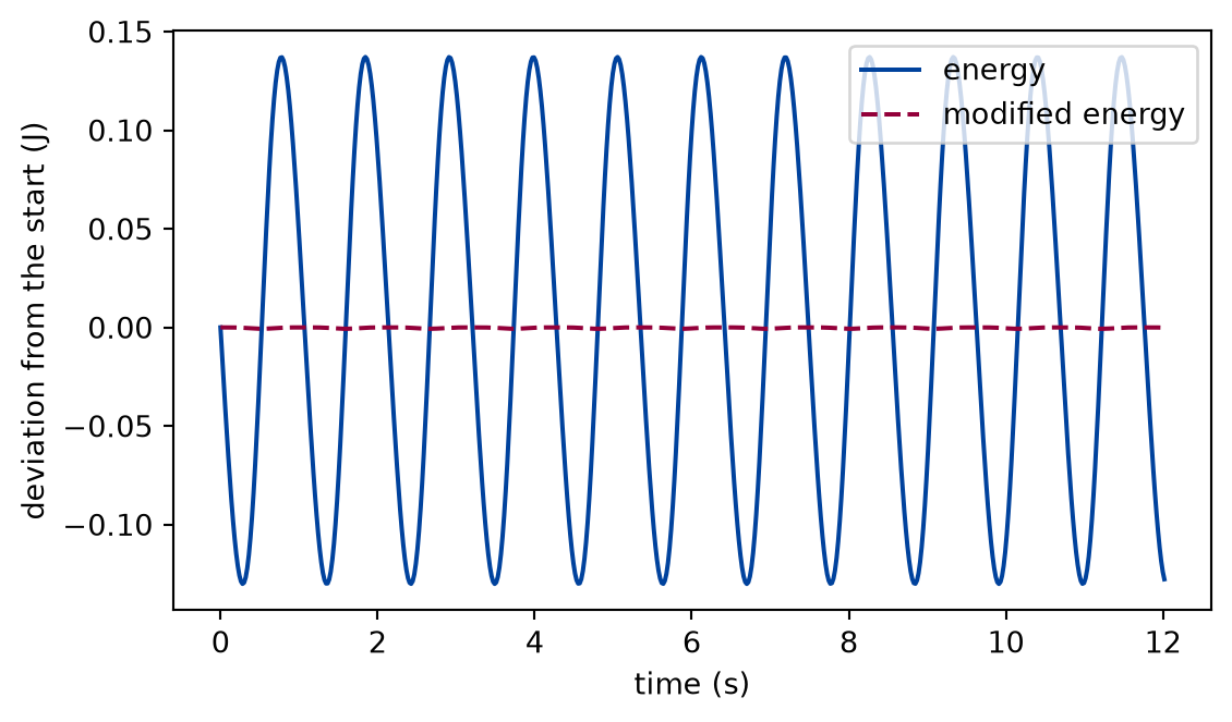
Numerically verified (the pendulum at one amplitude, twenty periods, three steps): The band of the energy shrinks by about a factor of two when the step is halved, as a first-order method, and the band of the modified energy by about a factor of four, as the first correction removed and the next left: the ratios are 2.00 and 4.00 at the finest step. The modified energy is conserved to a smaller band, not to round-off, which is what the second-order terms that were cut off say.

def draw_modified_energy_pendulum(runs) -> Figure:
    """The energy and the modified energy over six periods."""
    trajectory, energy, modified = runs[100]
    early = trajectory.t <= 6.0 * t0
    fig, ax = plt.subplots(figsize=(6.4, 3.6))
    ax.plot(
        trajectory.t[early],
        (energy - energy[0])[early],
        color=FIGURE_COLOURS[0],
        linestyle="-",
        label="energy",
    )
    ax.plot(
        trajectory.t[early],
        (modified - modified[0])[early],
        color=FIGURE_COLOURS[1],
        linestyle="--",
        label="modified energy",
    )
    ax.set_xlabel("time (s)")
    ax.set_ylabel("deviation from the start (J)")
    ax.legend(loc="upper right")
    return fig

src/pbc/mechanics/experiments/hamiltonian_mechanics.py, lines 296 to 318, read from the repository when this page was built.

Plot of energy minus its starting value, in joules, against time in seconds. The solid curve, the energy, oscillates up and down with the period of the pendulum within a band that is the same at the end as at the start. The dashed curve, the modified energy, lies close to zero with a much smaller oscillation. — Figure 2: simulated The energy and the modified energy of symplectic Euler on the pendulum over the first periods of the run at a hundred steps per period. The energy oscillates within a band that does not grow; the modified energy stays far closer to its starting value.

Limits

The modified energy is a truncated series. For the oscillator it ends after one term and is exact; for the pendulum it is conserved to second order in the step, as measured over twenty periods and three steps. That it stays that way over a very long run is the content of a theorem (backward error analysis) that holds for smooth potentials and small steps, and is not proved here.
The area is a measure for one degree of freedom. A system with more has a stronger condition than conserved volume, and a method can preserve volume without being symplectic.
A symplectic method keeps the energy bounded; it does not make it accurate. The width of the band is the first-order term for symplectic Euler, and the exercise shows that a higher-order method that is not symplectic can have a smaller error for a short run. The lesson does not tell where the crossing is for other systems.
Symplectic methods lose their properties with a variable step. The step map of a method that chooses its step from the state is not area-preserving, and the conserved energy is lost; a fixed step is assumed throughout.
The determinants and the areas are measured at a few states and one start. The argument for the shears is general, the measurements are not.
The Hamiltonian is obtained numerically, with the accuracy of the central differences of the previous lesson.

Self-check. A symplectic method keeps the energy within a band that does not grow, and a fourth-order method that is not symplectic has a far smaller error after a short run. A colleague concludes that the fourth-order method is always the better choice. What would you ask before agreeing, and what does the first exercise measure?

With scripts, you can record in this browser that you answered this question.

Solution to the self-check

Ask how long the run is. The error of a non-symplectic method of high order is small and grows without bound, steadily or in steps, while the error of the symplectic method is larger and stops growing. For a short run the first is smaller, and there is a run length after which the second is. So the question is the number of periods against the step, and the answer depends on both. The exercise finds that length for the pendulum at one step: the fourth-order method is better until its drift passes the band of velocity Verlet, and worse after it. If the run must be longer than that, or the property that the energy stays bounded is what is wanted, the symplectic method is the choice.

Exercises

Exercise 1. When is a symplectic method better? For the pendulum at an amplitude of one and a fifth radians, run velocity Verlet and the classical Runge-Kutta method at twenty steps per period for three hundred periods. After how many periods does the energy drift of the Runge-Kutta method pass the band of velocity Verlet?

Hint 1 of 2 for exercise 1

Take the running maximum of the deviation of the energy from its start for each method and find the first time the Runge-Kutta value is larger than the final value of the other.

Hint 2 of 2 for exercise 1

Convert the time to periods with the small-angle period, and expect the answer to depend on the step and the amplitude.

Solution to exercise 1

def long_run(experiment: Experiment) -> float:
    """Exercise 1: three hundred periods of the pendulum with velocity Verlet
    and Runge-Kutta 4; record the table and return the period, in
    small-angle periods, at which the drift of Runge-Kutta passes the band of
    Verlet."""
    steps = 20
    long_runs = {
        name: simulate(
            State(0.0, [1.2], [0.0]), pendulum, t0 / steps, 300 * steps, step=step
        )
        for name, step in (
            ("velocity Verlet", verlet_step),
            ("classical Runge-Kutta", rk4_step),
        )
    }
    drifts = {}
    for name, trajectory in long_runs.items():
        e = mechanical_energy(trajectory, 1.0, potential_p)
        drifts[name] = np.maximum.accumulate(np.abs(e - e[0]) / abs(e[0]))
    band = drifts["velocity Verlet"][-1]
    crossing = (
        long_runs["velocity Verlet"].t[
            np.argmax(drifts["classical Runge-Kutta"] > band)
        ]
        / t0
    )

    experiment.table(
        "long-run",
        [
            (
                "velocity Verlet",
                drifts["velocity Verlet"][len(drifts["velocity Verlet"]) // 30],
                band,
            ),
            (
                "classical Runge-Kutta",
                drifts["classical Runge-Kutta"][
                    len(drifts["classical Runge-Kutta"]) // 30
                ],
                drifts["classical Runge-Kutta"][-1],
            ),
        ],
        columns=[
            ("method", "", ""),
            ("drift after ten periods", "", ".1e"),
            ("drift after three hundred periods", "", ".1e"),
        ],
        caption="The largest relative deviation of the energy from its start for "
        "velocity Verlet and the classical Runge-Kutta method, after ten and after "
        "three hundred periods of the pendulum at twenty steps per period.",
    )
    return crossing

src/pbc/mechanics/experiments/hamiltonian_mechanics.py, lines 321 to 373, read from the repository when this page was built.

The largest relative deviation of the energy from its start for velocity Verlet and the classical Runge-Kutta method, after ten and after three hundred periods of the pendulum at twenty steps per period.
method	drift after ten periods	drift after three hundred periods
velocity Verlet	2.2e-02	2.2e-02
classical Runge-Kutta	1.7e-03	5.0e-02

The Runge-Kutta drift grows with every period and passes the whole band of velocity Verlet after about 130 periods; before that it is the smaller of the two, as the first row says. With a finer step both change, and the crossing moves to a longer run, which is why the answer is a number for this step and not a rule.

Exercise 2. The sign of the correction. The modified energy of symplectic Euler as written in the lesson subtracts $\tfrac12\Delta t\,U' v$ . Add it instead, and compare the band of the result with the band of the energy over twenty periods of the oscillator at sixteen steps per period.

Hint 1 of 1 for exercise 2

The two corrections differ in sign. Which one cancels the oscillation of the energy, and which doubles it?

Solution to exercise 2

def sign_of_the_correction(experiment: Experiment, se_run) -> float:
    """Exercise 2: the spread of the energy with the correction subtracted
    and added; record the table and return the spread with the wrong sign
    over that of the energy."""
    wrong = mechanical_energy(se_run, mass, potential) + 0.5 * dt * np.array(
        [gradient(x) @ v for x, v in zip(se_run.x, se_run.v, strict=True)]
    )
    right = symplectic_euler_modified_energy(se_run, mass, potential, gradient, dt)
    plain = mechanical_energy(se_run, mass, potential)

    experiment.table(
        "sign-of-the-correction",
        [
            ("energy", spread(plain)),
            ("minus the correction", spread(right)),
            ("plus the correction", spread(wrong)),
        ],
        columns=[("quantity", "", ""), ("spread", "", ".1e")],
        caption="The spread of the energy and of the energy with the correction of "
        "the explanation subtracted and added, symplectic Euler on the "
        "oscillator.",
    )
    return spread(wrong) / spread(plain)

src/pbc/mechanics/experiments/hamiltonian_mechanics.py, lines 376 to 398, read from the repository when this page was built.

The spread of the energy and of the energy with the correction of the explanation subtracted and added, symplectic Euler on the oscillator.
quantity	spread
energy	2.4e-01
minus the correction	2.2e-15
plus the correction	4.9e-01

Subtracting it removes the oscillation to round-off. Adding it makes the band wider than that of the energy itself, by a factor of about 2.0. The sign is not a convention: the correction is the cross term that the update leaves in the energy, and only the right sign cancels it.

Run this experiment

This page was built from commit 6417e2ff90258bd2d2ba21d217eb7666fd24f680 of the repository.

In a clone at that commit, with the project’s Python packages installed, this command runs the experiment of this page:

uv run --locked --no-dev python -m pbc.mechanics.experiments.hamiltonian_mechanics results

Files, tests, and every command

The files behind it:

site/lessons/mechanics/15-hamiltonian-mechanics/index.qmd: this page, with every code cell.
src/pbc/mechanics/dynamics.py: code the experiment runs.
src/pbc/mechanics/integrators.py: code the experiment runs.
src/pbc/mechanics/energy.py: code the experiment runs.
src/pbc/mechanics/lagrangian.py: code the experiment runs.
src/pbc/mechanics/hamiltonian.py: code the experiment runs.
src/pbc/mechanics/pendulum.py: code the experiment runs.
src/pbc/mechanics/oscillator.py: code the experiment runs.
src/pbc/mechanics/experiments/hamiltonian_mechanics.py: code the experiment runs.
src/pbc/experiment.py: code the experiment runs.
tests/unit/test_integrators.py: tests of that code.
tests/unit/test_energy.py: tests of that code.
tests/unit/test_lagrangian.py: tests of that code.
tests/unit/test_hamiltonian.py: tests of that code.
tests/unit/test_pendulum.py: tests of that code.
tests/unit/test_hamiltonian_mechanics_experiment.py: tests of that code.

With Git and uv installed (see the setup page), run:

git clone https://github.com/taspinar/physics-by-construction.git
cd physics-by-construction
git checkout 6417e2ff90258bd2d2ba21d217eb7666fd24f680
uv sync --locked --no-dev
uv run --locked --no-dev python -m pbc.mechanics.experiments.hamiltonian_mechanics results

The experiment writes every figure of this page into results/, as <label>.png, and every number and table of the page, as the page shows it, into results/results.json. Its numbers match this page to the digits shown, and its figure files are the ones the page shows; digits beyond those can differ between machines, because floating-point libraries differ. Change the code of the experiment and run it again to see what changes.