Random walks and diffusion

A walker that takes one random step at a time, the diffusion law that many of them obey, and the diffusion coefficient measured from the walk and checked against the value the step rule predicts.

Course

Thermodynamics and statistical physics, lesson 2 of 4

Slot

T1, Random walks and diffusion

Methods

Simulation

Difficulty

Introductory, level 1 of 3

What you’ll learn

Build a random walk from one rule for a single step
Measure the mean squared displacement of many walkers and the diffusion coefficient it gives
Check the measured coefficient and the spread of the walkers against what the step rule predicts

Prerequisites

Kinematics as a program.

Before you begin

Statistics: the mean, the variance, and the standard error of a mean
Probability: independent random variables, and the Gaussian distribution

Related

none

Previous

Resonance and driven oscillators

Next

Kinetic theory of gases

With scripts, this page keeps a record in your browser of whether you completed the lesson. Nothing is stored without them.

With scripts, this place suggests what to do next, with the reason, from the progress saved in your browser. Without them, follow the learning path.

A drop of ink in still water spreads, though no current carries it. A smell crosses a room faster than the air moves. Nothing pushes the ink or the smell in any direction: each molecule is knocked about by its neighbours, and the spreading belongs to the crowd. How fast does the crowd spread, and what does that speed have to do with the knocks?

This lesson builds the smallest model of the knocks: a walker that takes one step of a fixed length in a random direction, again and again, each step independent of the last. It is the state and the update rule of the kinematics lesson, with a random velocity in place of a given one. No rule mentions spreading. The lesson then measures how far many walkers have gone from the start, finds that the square of the distance grows in proportion to the time, and reads off a diffusion coefficient. The step rule predicts that coefficient, so the measurement has something to be checked against. The checks are statistical, because the walk is random, and they use the tolerance of the gas lesson: four standard errors over independent runs. The data are simulated; no real ink is measured.

Assumptions

Equal steps at equal times. Every step has the same length $\ell$ and takes the same time $\tau$ . Real molecules have a spread of free paths and of times between collisions. The coefficient below then depends on the mean squared step and the mean time, which is what the formula uses when the steps are equal.
Directions are uniform and independent. Each step points in a direction drawn uniformly from the circle, whatever the earlier steps were. A walker that tends to continue in the direction it was going (a persistent walk) spreads faster than this formula says, and a walker that is pulled back to a point does not spread without limit.
No walker affects another. The walkers do not collide and do not see each other, so the average over them is an average over independent copies. A crowd that excludes itself (a dense gas) has a different diffusion coefficient for the same step.
Many steps. The diffusion law and the Gaussian spread are the limit of many steps. After a few steps the walkers sit on a few circles around the start, and the Gaussian is a poor description.
Randomness is seeded. A generator created from a seed makes the walks, so a run is a function of its inputs and the page is the same at every build.
The runs are independent, the steps are not walkers. The standard error of a measured quantity is computed from the spread between independent runs with different seeds. The walkers inside one run are independent too, but a quantity that is read off one walker at successive times is correlated with itself, and the lesson never treats those readings as independent.

Explanation

From one rule to the mean squared displacement

The state of a walker is its position $\mathbf r_n$ after $n$ steps. One step is

$\mathbf r_{n+1} = \mathbf r_n + \ell\,\hat{\mathbf e}_n,$

with $\hat{\mathbf e}_n$ a unit vector in a random direction. Start at the origin and add the steps: $\mathbf r_n = \ell\sum_{k<n}\hat{\mathbf e}_k$ . The square of the distance is the sum of every product of two steps,

$\lvert\mathbf r_n\rvert^2 = \ell^2\sum_{j<n}\sum_{k<n}\hat{\mathbf e}_j\cdot\hat{\mathbf e}_k .$

The mean of $\hat{\mathbf e}_j\cdot\hat{\mathbf e}_k$ over independent uniform directions is zero when $j \neq k$ , because a direction and its opposite are equally likely, and it is one when $j = k$ . Only the $n$ terms of the diagonal survive:

$\langle r^2\rangle = n\,\ell^2 = \frac{\ell^2}{\tau}\,t, \qquad t = n\tau .$

The mean squared displacement grows in proportion to time. That is the diffusion law, and it is a property of the crowd: the distance of one walker grows like $\sqrt{t}$ on average, not like $t$ .

The diffusion coefficient

In $d$ dimensions the law is written $\langle r^2\rangle = 2\,d\,D\,t$ , which defines the diffusion coefficient $D$ . With the result above,

$D = \frac{\ell^2}{2\,d\,\tau},$

so in the plane $D = \ell^2/(4\tau)$ . The coefficient has the unit of $\mathrm{m^2/s}$ , and it is the only number the law needs: a larger step or a shorter time between steps spreads the walkers faster.

The shape of the spread

Each coordinate of $\mathbf r_n$ is a sum of many independent terms of mean zero, so for many steps it is Gaussian by the central limit theorem, with variance $\langle x^2\rangle = \langle r^2\rangle/2 = 2Dt$ in the plane. The distance $r$ then follows the Rayleigh distribution, and the probability that a walker is within a radius $R$ of the start is the integral of the Gaussian over the disc,

$P(r \le R) = 1 - \exp\!\left(-\frac{R^2}{4Dt}\right).$

This is a second check, on the shape and not only on the second moment. It uses the same $D$ .

What the tolerance means

A run gives one value of $D$ and another seed gives another. With $k$ independent runs, the mean estimates $D$ and the standard error $s/\sqrt{k}$ , with $s$ the sample standard deviation, says how far the mean is likely to be from the value the model gives for unlimited runs. A result agrees with the prediction within $4$ standard errors if the difference is at most $4$ times the standard error. Four is a chosen tolerance, not a law, and with only six runs the standard error is itself uncertain, so the discrepancy follows a Student $t$ distribution with five degrees of freedom: chance alone exceeds four standard errors in about one case in a hundred. A failure is a reason to look at the model or the program, and a repeat with other seeds tells the two apart. A model that is wrong by more than the tolerance is caught, and one that is wrong by less is not.

Code

The walk is pbc.thermodynamics.diffusion. random_walks draws every step of every walker at once from a seeded generator, and mean_squared_displacement averages the squared distance over the walkers.

def random_walks(
    n_walkers: int,
    n_steps: int,
    step_length: float,
    rng: np.random.Generator,
    dimension: int = 2,
) -> Array:
    """The positions (m) of ``n_walkers`` walkers that start at the origin,
    after 0, 1, ..., ``n_steps`` steps: an array of shape
    ``(n_steps + 1, n_walkers, dimension)``.

    Each step has length ``step_length`` and a direction uniform on the circle
    (``dimension`` 2) or on the line (``dimension`` 1, a step left or right).
    """
    if n_walkers < 1 or n_steps < 1 or step_length <= 0:
        raise ValueError(
            "n_walkers and n_steps must be at least 1, step_length positive"
        )
    if dimension == 1:
        steps = rng.choice([-1.0, 1.0], size=(n_steps, n_walkers, 1))
    elif dimension == 2:
        angles = rng.uniform(0.0, 2.0 * np.pi, size=(n_steps, n_walkers))
        steps = np.stack([np.cos(angles), np.sin(angles)], axis=-1)
    else:
        raise ValueError("dimension must be 1 or 2")
    paths = np.zeros((n_steps + 1, n_walkers, dimension))
    paths[1:] = np.cumsum(step_length * steps, axis=0)
    return paths

src/pbc/thermodynamics/diffusion.py, lines 20 to 47, read from the repository when this page was built.

The coefficient is the slope of $\langle r^2\rangle$ against time, through the origin and divided by $2d$ , and the prediction is a function too, so that the page and the tests compare with the same code.

def diffusion_coefficient(times: Array, msd: Array, dimension: int = 2) -> float:
    """The diffusion coefficient D (m²/s) from <r²> = 2 d D t: the slope of the
    least-squares line through the origin, divided by 2 d."""
    t = np.asarray(times, dtype=np.float64)
    slope = float(np.sum(t * msd) / np.sum(t * t))
    return slope / (2.0 * dimension)

src/pbc/thermodynamics/diffusion.py, lines 55 to 60, read from the repository when this page was built.

def predicted_diffusion_coefficient(
    step_length: float, tau: float, dimension: int = 2
) -> float:
    """D = l² / (2 d tau) (m²/s) for steps of length l every tau seconds: the
    steps are independent with mean square l², so <r²> = n l² after n steps,
    that is l² t / tau."""
    return step_length**2 / (2.0 * dimension * tau)

src/pbc/thermodynamics/diffusion.py, lines 63 to 69, read from the repository when this page was built.

Worked examples

The mean squared displacement grows with time

The walkers take steps of 0.1 m every 0.5 s. Each run follows 500 walkers for 200 steps and records $\langle r^2\rangle$ after every step; six runs with different seeds are made.

STEP = 0.1  # step length, m
TAU = 0.5  # time between steps, s
N_WALKERS = 500
N_STEPS = 200
SEEDS = range(6)

times = TAU * np.arange(N_STEPS + 1)
predicted_d = predicted_diffusion_coefficient(STEP, TAU)

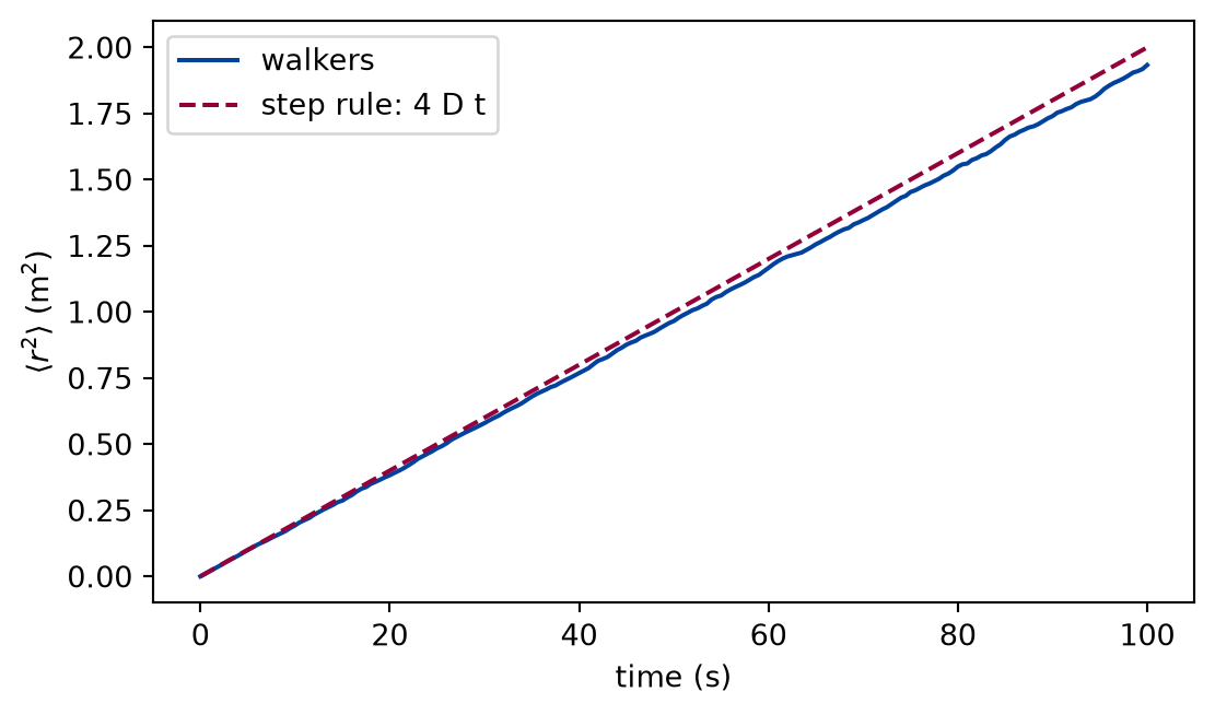
src/pbc/thermodynamics/experiments/random_walks_and_diffusion.py, lines 31 to 38, read from the repository when this page was built.

def msd_run(experiment: Experiment):
    """Six runs of the walkers, their mean squared displacement, and the
    table of three times against the step rule."""
    runs = [
        random_walks(N_WALKERS, N_STEPS, STEP, np.random.default_rng(seed))
        for seed in SEEDS
    ]
    msds = np.array([mean_squared_displacement(paths) for paths in runs])
    msd = msds.mean(axis=0)

    checkpoints = [N_STEPS // 4, N_STEPS // 2, N_STEPS]
    experiment.table(
        "msd-run",
        [(n, times[n], msd[n], 4.0 * predicted_d * times[n]) for n in checkpoints],
        [
            ("steps", "", "d"),
            ("time", "s", ".1f"),
            ("measured <r²>", "m²", ".3f"),
            ("predicted 4 D t", "m²", ".3f"),
        ],
        "The mean squared displacement averaged over six runs of the walkers, at "
        "three times, against the prediction of the step rule.",
    )
    return runs, msds, msd

src/pbc/thermodynamics/experiments/random_walks_and_diffusion.py, lines 42 to 65, read from the repository when this page was built.

The mean squared displacement averaged over six runs of the walkers, at three times, against the prediction of the step rule.
steps	time (s)	measured <r²> (m²)	predicted 4 D t (m²)
50	25.0	0.484	0.500
100	50.0	0.965	1.000
200	100.0	1.933	2.000

def draw_msd(msd) -> Figure:
    """The mean squared displacement against time, with the step rule."""
    fig, ax = plt.subplots(figsize=(6.4, 3.6))
    ax.plot(times, msd, color="#00429d", label="walkers")
    ax.plot(
        times,
        4.0 * predicted_d * times,
        color="#93003a",
        linestyle="--",
        label="step rule: 4 D t",
    )
    ax.set_xlabel("time (s)")
    ax.set_ylabel(r"$\langle r^2\rangle$ (m$^2$)")
    ax.legend()
    return fig

src/pbc/thermodynamics/experiments/random_walks_and_diffusion.py, lines 68 to 82, read from the repository when this page was built.

Line plot of the mean squared displacement in square metres against time in seconds. The measured curve rises almost straight from the origin, and a dashed straight line from the origin lies on top of it. — Figure 1: simulated The mean squared displacement of the walkers grows in a straight line with time, along the line the step rule predicts. The spread between the six runs is too small to see at this scale.

The table and the figure show one thing: the squared distance is proportional to the time, and the line is the one the step rule gives, $4Dt$ with $D = \ell^2/(4\tau)$ , not one fitted to the data. The data are simulated, and the check is the prediction of the model that made them.

The diffusion coefficient against the step rule

Each of the six runs gives its own coefficient from the slope of its own $\langle r^2\rangle$ . The mean over the runs and its standard error are compared with the prediction.

def diffusion_check(experiment: Experiment, msds):
    """The diffusion coefficient of each run, their mean, and its distance in
    standard errors from the step rule and from a wrong prediction; record
    the table of the runs."""
    estimates = np.array([diffusion_coefficient(times, row) for row in msds])
    mean_d, error_d = mean_and_error(estimates)
    off = abs(mean_d - predicted_d) / error_d
    wrong = abs(mean_d - 2.0 * predicted_d) / error_d

    experiment.table(
        "diffusion-check",
        list(zip(SEEDS, estimates, strict=True)),
        [("seed", "", "d"), ("D", "m²/s", ".5f")],
        "The diffusion coefficient measured in each of the six runs.",
    )
    return mean_d, error_d, off, wrong

src/pbc/thermodynamics/experiments/random_walks_and_diffusion.py, lines 85 to 100, read from the repository when this page was built.

The diffusion coefficient measured in each of the six runs.
seed	D (m²/s)
0	0.00467
1	0.00467
2	0.00497
3	0.00475
4	0.00494
5	0.00498

The mean of the six measured coefficients, its standard error, and its distance in standard errors from the step rule and from a wrong prediction.
compared with	mean D (m²/s)	standard error (m²/s)	prediction (m²/s)	difference (standard errors)
step rule	0.00483	0.00006	0.00500	2.8
a coefficient twice as large	0.00483	0.00006	0.01000	84.2

Numerically verified (equal steps in the plane, six runs of five hundred walkers, four standard errors): The diffusion coefficient measured from the mean squared displacement agrees with $\ell^2/(4\tau)$ within the tolerance of four standard errors, and a prediction twice as large is rejected. The measured coefficient is 0.00483 $\mathrm{m^2/s}$ with a standard error of 0.00006 $\mathrm{m^2/s}$ , 2.8 standard errors from the prediction of 0.00500 $\mathrm{m^2/s}$ . The wrong prediction is 84 standard errors away, so the check can tell the two apart.

The Gaussian spread

The mean squared displacement tests the second moment only. The probability that a walker is within a radius of the start tests the shape. Take the radius that the prediction says contains half of the walkers after the last step, and count.

def radial_check(experiment: Experiment, runs) -> list:
    """The fraction of walkers within three radii after the last step against
    the Gaussian prediction; record the table and return its rows."""
    t_end = times[-1]
    radii = np.sqrt(
        4.0 * predicted_d * t_end * -np.log(1.0 - np.array([0.25, 0.5, 0.75]))
    )
    rows = []
    for radius in radii:
        measured = np.array([fraction_within(paths[-1], radius) for paths in runs])
        mean_f, error_f = mean_and_error(measured)
        predicted_f = predicted_fraction_within(radius, predicted_d, t_end)
        rows.append(
            (radius, mean_f, error_f, predicted_f, abs(mean_f - predicted_f) / error_f)
        )

    experiment.table(
        "radial-check",
        rows,
        [
            ("radius", "m", ".2f"),
            ("measured fraction", "", ".3f"),
            ("standard error", "", ".3f"),
            ("predicted fraction", "", ".3f"),
            ("difference", "standard errors", ".1f"),
        ],
        "The fraction of walkers within three radii after the last step, over six "
        "runs, against the Gaussian prediction.",
    )
    return rows

src/pbc/thermodynamics/experiments/random_walks_and_diffusion.py, lines 125 to 154, read from the repository when this page was built.

The fraction of walkers within three radii after the last step, over six runs, against the Gaussian prediction.
radius (m)	measured fraction	standard error	predicted fraction	difference (standard errors)
0.76	0.257	0.007	0.250	1.0
1.18	0.510	0.006	0.500	1.7
1.67	0.764	0.008	0.750	1.7

Numerically verified (the last step of the walk, six runs, four standard errors): The fraction of walkers within a radius agrees with $1 - \exp(-R^2/4Dt)$ at three radii within four standard errors. The largest difference is 1.7 standard errors. The two checks use the same $D$ , so together they say that the walkers spread by the law and in the shape that the step rule predicts.

Limits

A model checked against a prediction, not against ink. The data are simulated from the rule that the prediction is derived from. The result says that the program implements the rule and that the derivation is right for it. It does not say that molecules take equal steps; no measurement is involved, so no claim here is experimentally supported.
What the tolerance can see. A coefficient wrong by more than four standard errors is caught, and a smaller error is not. Agreement of a second moment and three fractions is a test of the shape in four places, not a proof of it.
The plane. The numbers are for two dimensions. The formula $D = \ell^2/(2d\tau)$ is stated for one and two dimensions, and the unit tests check both; the lesson shows only the plane.
Only the long-time law. The linear growth is exact for equal independent steps at every step count, but the Gaussian shape is a limit of many steps.
No physics of the molecule. What sets $\ell$ and $\tau$ in a real liquid is not modelled. They are the two numbers the walk takes as given.

Self-check. The mean squared displacement of the walkers is a straight line in time. Does that show that every walker moves in a straight line at a fixed speed?

Yes: a straight line in $\langle r^2\rangle$ means a constant speed.

No. A walker that moves at a constant speed has $r = vt$ , so $\langle r^2\rangle = v^2t^2$ , which grows as the square of the time.
No: the line is in the average of the squared distance, and each walker’s distance grows only like the square root of time.

Right. The average of the square grows in proportion to $t$ because the cross terms between different steps cancel, so the typical distance grows like $\sqrt{t}$ , slower than a straight line.

Solution to the self-check

The linear growth of $\langle r^2\rangle$ is the signature of independent random steps, as the derivation shows. Motion at a constant velocity gives $\langle r^2\rangle \propto t^2$ , and a walker held near a point gives a $\langle r^2\rangle$ that stops growing. The exponent of time in $\langle r^2\rangle$ tells these motions apart.

Exercises

Exercise 1. A doubled step. Run the walk with a step twice as long and the same time between steps. By what factor does the measured diffusion coefficient change, and what does the step rule predict?

Hint 1 of 1 for exercise 1

The coefficient depends on the step through its square.

Solution to exercise 1

The prediction is $\ell^2/(4\tau)$ , so doubling $\ell$ multiplies it by four.

def doubled_step(experiment: Experiment, mean_d) -> None:
    """Exercise 1: the diffusion coefficient of the doubled step in units of
    the first; record the table."""
    doubled = [
        random_walks(N_WALKERS, N_STEPS, 2.0 * STEP, np.random.default_rng(seed))
        for seed in SEEDS
    ]
    doubled_d = np.array(
        [diffusion_coefficient(times, mean_squared_displacement(p)) for p in doubled]
    )
    mean_2, error_2 = mean_and_error(doubled_d)
    experiment.table(
        "doubled-step",
        [(mean_2 / mean_d, 4.0, error_2 / mean_d)],
        [
            ("measured ratio", "", ".2f"),
            ("predicted ratio", "", ".1f"),
            ("standard error of the ratio", "", ".2f"),
        ],
        "The measured diffusion coefficient of the doubled step in units of the "
        "first, with the predicted ratio.",
    )

src/pbc/thermodynamics/experiments/random_walks_and_diffusion.py, lines 157 to 178, read from the repository when this page was built.

The measured diffusion coefficient of the doubled step in units of the first, with the predicted ratio.
measured ratio	predicted ratio	standard error of the ratio
4.00	4.0	0.05

The ratio is within a few standard errors of the prediction.

Exercise 2. One dimension. Walk on a line, each step to the left or to the right. What is $D$ for the same $\ell$ and $\tau$ , and does the measurement agree?

Solution to exercise 2

In one dimension $\langle x^2\rangle = 2Dt$ and $\langle x^2\rangle = \ell^2 t/\tau$ , so $D = \ell^2/(2\tau)$ , twice the value in the plane for the same step.

def on_a_line(experiment: Experiment) -> None:
    """Exercise 2: the diffusion coefficient of walkers on a line; record the
    table."""
    line = [
        diffusion_coefficient(
            times,
            mean_squared_displacement(
                random_walks(
                    N_WALKERS, N_STEPS, STEP, np.random.default_rng(seed), dimension=1
                )
            ),
            dimension=1,
        )
        for seed in SEEDS
    ]
    mean_1, error_1 = mean_and_error(np.array(line))
    predicted_1 = predicted_diffusion_coefficient(STEP, TAU, dimension=1)
    experiment.table(
        "on-a-line",
        [(mean_1, error_1, predicted_1, abs(mean_1 - predicted_1) / error_1)],
        [
            ("measured D", "m²/s", ".5f"),
            ("standard error", "m²/s", ".5f"),
            ("predicted D", "m²/s", ".5f"),
            ("difference", "standard errors", ".1f"),
        ],
        "The diffusion coefficient of walkers on a line, over six runs, against "
        "the prediction.",
    )

src/pbc/thermodynamics/experiments/random_walks_and_diffusion.py, lines 181 to 209, read from the repository when this page was built.

The diffusion coefficient of walkers on a line, over six runs, against the prediction.
measured D (m²/s)	standard error (m²/s)	predicted D (m²/s)	difference (standard errors)
0.00975	0.00025	0.01000	1.0

Run this experiment

This page was built from commit 6417e2ff90258bd2d2ba21d217eb7666fd24f680 of the repository.

In a clone at that commit, with the project’s Python packages installed, this command runs the experiment of this page:

uv run --locked --no-dev python -m pbc.thermodynamics.experiments.random_walks_and_diffusion results

Files, tests, and every command

The files behind it:

site/lessons/thermodynamics/01-random-walks-and-diffusion/index.qmd: this page, with every code cell.
src/pbc/thermodynamics/diffusion.py: code the experiment runs.
src/pbc/thermodynamics/experiments/random_walks_and_diffusion.py: code the experiment runs.
src/pbc/experiment.py: code the experiment runs.
tests/unit/test_thermodynamics.py: tests of that code.
tests/unit/test_random_walks_and_diffusion_experiment.py: tests of that code.

With Git and uv installed (see the setup page), run:

git clone https://github.com/taspinar/physics-by-construction.git
cd physics-by-construction
git checkout 6417e2ff90258bd2d2ba21d217eb7666fd24f680
uv sync --locked --no-dev
uv run --locked --no-dev python -m pbc.thermodynamics.experiments.random_walks_and_diffusion results

The experiment writes every figure of this page into results/, as <label>.png, and every number and table of the page, as the page shows it, into results/results.json. Its numbers match this page to the digits shown, and its figure files are the ones the page shows; digits beyond those can differ between machines, because floating-point libraries differ. Change the code of the experiment and run it again to see what changes.