Resonance and driven oscillators

A damped oscillator pushed at a steady rhythm: the amplitude and phase that it settles into, the resonance curve with its peak and width, and a simulation of the whole curve validated against the analytic amplitude.

Course

Classical mechanics, lesson 12 of 28

Slot

M12, Resonance and driven oscillators

Methods

Simulation

Difficulty

Intermediate, level 2 of 3

What you’ll learn

Write the damped, driven oscillator and its steady-state amplitude and phase
Read the peak, the width, and the quality factor off a resonance curve
Simulate the curve and validate it against the analytic amplitude, with the transient separated from the steady state
Say how long a driven system takes to settle and why a larger quality factor takes longer

Prerequisites

The harmonic oscillator, Projectile motion with quadratic drag, Numerical integrators.

Before you begin

Calculus: derivatives, and the maximum of a function found where its derivative is zero
Complex numbers: the exponential of an imaginary number, and the modulus and argument of a complex ratio
Trigonometry: the amplitude and phase of a sum of a sine and a cosine of the same frequency

Related

none

Previous

Hamiltonian mechanics

Next

Random walks and diffusion

With scripts, this page keeps a record in your browser of whether you completed the lesson. Nothing is stored without them.

With scripts, this place suggests what to do next, with the reason, from the progress saved in your browser. Without them, follow the learning path.

A child on a swing is pushed once per swing and the swing rises; pushed at the wrong rhythm it hardly moves. A wine glass sings when a voice reaches its pitch. A radio picks one station out of thousands by tuning a circuit until it answers to that frequency alone, and a bridge, a building, and the atoms of a gas in a field all answer most strongly to a rhythm of their own. The same equation describes them: an oscillator with some friction, driven by a force that varies sinusoidally in time. The question of the lesson is what such a system does in the long run, how much it moves, at what delay behind the push, and how sharply it prefers one rhythm over the others.

The lesson solves the problem in closed form, since the equation is linear, then simulates the response over a whole range of driving frequencies with the classical Runge-Kutta method and validates the simulated curve against the closed form: the resonance curve is a check of the program as much as a result of the physics. The code lives in pbc.mechanics.resonance, the reference solution of the damped driven oscillator that the coding-agent exercise on simulation development, built on the same equation, reuses.

Assumptions

The model and the program rest on these assumptions. Each one names what goes wrong when it does not hold.

Hooke’s law. The spring force is proportional to the displacement, so the equation is linear and the response to a sinusoid is a sinusoid at the same frequency. A spring that stiffens or softens with the stretch bends the resonance curve and can make it jump between two amplitudes; that belongs to the lesson on nonlinear dynamics.
Linear drag. The damping force is proportional to the velocity, as in the drag lesson at low speed. Friction of another kind, such as dry friction or quadratic drag, changes the shape of the peak and the closed form no longer holds.
A sinusoidal force of fixed amplitude. The driving force is $F_0\cos\Omega t$ with a constant amplitude and frequency. A drive whose amplitude depends on the response, as a motor that slows when loaded does, is a different problem.
One degree of freedom. One mass, one spring. A structure with several masses has several resonances, one per normal mode, as the coupled springs of the Lagrangian lesson have.
Underdamped for the closed form of the transient. The exact motion from rest is given for damping below the critical value. The steady-state results hold for any damping.
The step resolves the driving period, and the run outlasts the transient. The simulation takes many steps per driving period and runs for several decay times before the amplitude is read, so that what is measured is the steady state and not the start.

The driven oscillator

The equation and its scales

A mass $m$ on a spring $k$ , with the drag $-b v$ and the force $F_0\cos\Omega t$ , obeys Newton’s second law,

$m\ddot x = -k x - b\,\dot x + F_0 \cos\Omega t .$

Divide by the mass and define the natural angular frequency $\omega_0 = \sqrt{k/m}$ and the damping rate $\gamma = b/(2m)$ :

$\ddot x + 2\gamma\,\dot x + \omega_0^2\,x = \frac{F_0}{m}\cos\Omega t .$

Without the force the motion is a decaying oscillation, $e^{-\gamma t}\cos\omega_d t$ with $\omega_d = \sqrt{\omega_0^2 - \gamma^2}$ , as the amplitude falls by a factor of $e$ every $1/\gamma$ seconds. The quality factor

$Q = \frac{\omega_0}{2\gamma} = \frac{\sqrt{k m}}{b}$

is the number of radians the free motion covers while its energy falls by a factor of $e$ : a large $Q$ is a system that rings for many swings.

The steady state

The equation is linear, so its solution is a particular solution that follows the force plus a free motion that decays. After the free part has gone, the mass moves at the driving frequency. Write the force as the real part of $(F_0/m)\,e^{i\Omega t}$ and look for the motion as the real part of $\tilde A\,e^{i\Omega t}$ with a complex amplitude $\tilde A$ . Each derivative brings a factor of $i\Omega$ , so

$\bigl(\omega_0^2 - \Omega^2 + 2 i\gamma\Omega\bigr)\,\tilde A = \frac{F_0}{m}, \qquad \tilde A = \frac{F_0/m}{\omega_0^2 - \Omega^2 + 2 i\gamma\Omega}.$

The modulus of $\tilde A$ is the amplitude $A$ of the motion, and the argument is minus the delay of the motion behind the force, $x = A\cos(\Omega t - \delta)$ :

$A(\Omega) = \frac{F_0/m}{\sqrt{(\omega_0^2 - \Omega^2)^2 + 4\gamma^2\Omega^2}}, \qquad \delta(\Omega) = \operatorname{atan2}\bigl(2\gamma\Omega,\ \omega_0^2 - \Omega^2\bigr).$

For a slow drive, $\Omega \ll \omega_0$ , the amplitude is the static displacement $F_0/k$ and the delay is zero: the mass follows the force. For a fast drive the amplitude falls as $1/\Omega^2$ and the delay approaches half a turn: the mass is pushed the wrong way for the whole swing. At $\Omega = \omega_0$ the delay is a quarter of a turn whatever the damping, and the amplitude is $F_0/(2\gamma m\omega_0) = Q F_0/k$ : the static displacement times $Q$ .

The peak and the width

The amplitude is largest where the denominator under the root is smallest. Setting the derivative of $(\omega_0^2 - \Omega^2)^2 + 4\gamma^2\Omega^2$ with respect to $\Omega^2$ to zero gives the peak frequency

$\Omega_r = \sqrt{\omega_0^2 - 2\gamma^2},$

a little below the natural frequency, and it exists only for $2\gamma^2 < \omega_0^2$ ; for more damping the response only falls. For a small $\gamma$ the peak is at $\omega_0$ to a good approximation, with the height $Q F_0/k$ .

Power is what the system absorbs: on the average the drag takes $\tfrac12 b\,\Omega^2 A^2$ , which is proportional to $A^2\Omega^2$ . For weak damping the power falls to half its peak value at $\Omega \approx \omega_0 \pm \gamma$ , so the full width at half power is

$\Delta\omega \approx 2\gamma = \frac{b}{m}, \qquad Q = \frac{\omega_0}{\Delta\omega}.$

The quality factor is thus also the sharpness of the resonance: the peak frequency divided by its width. A tuner with a large $Q$ separates stations that are close in frequency and takes a long time to settle on one.

The transient

The complete motion from the start $(x_0, v_0)$ is the steady state plus a free motion that fits the start, so that the position and the velocity are right at the first instant:

$x(t) = A\cos(\Omega t - \delta) + e^{-\gamma t}\bigl(C_1\cos\omega_d t + C_2\sin\omega_d t\bigr).$

The two constants follow from $x_0$ and $v_0$ (the program does it). The free part decays by a factor of $e$ in $1/\gamma = 2Q/\omega_0$ , so the time to settle is proportional to $Q$ . When the drive is near the natural frequency the free part and the steady state have close frequencies, and their sum beats while the free part dies away.

The program

The reusable code is pbc.mechanics.resonance. The driving force is an extra force for the Newton model of the earlier lessons, next to the spring and the linear drag; the rest is the reference solution.

def driving_force(amplitude: float, omega: float) -> Force:
    """The force F₀ cos(Ω t) in N, with the ``amplitude`` F₀ (N) and the
    angular frequency ``omega`` Ω (rad/s), along every coordinate."""

    def force(t: float, x: Vector, v: Vector) -> Vector:
        return np.full_like(x, amplitude * np.cos(omega * t))

    return force

src/pbc/mechanics/resonance.py, lines 40 to 47, read from the repository when this page was built.

The closed forms of the steady state:

def steady_state_amplitude(
    mass: float, k: float, b: float, force: float, omega: ArrayLike
) -> NDArray[np.float64]:
    """The amplitude in m of the motion at the driving frequency ``omega``
    (rad/s) after the transient, for the force amplitude ``force`` (N):
    (F₀ / m) / sqrt((ω₀² - Ω²)² + 4 gamma² Ω²)."""
    _check(mass, k, b)
    omega = np.asarray(omega, dtype=np.float64)
    w0sq, gamma = k / mass, damping_rate(mass, b)
    return (force / mass) / np.sqrt((w0sq - omega**2) ** 2 + 4.0 * gamma**2 * omega**2)

Line 80, return (force / mass) / np.sqrt((w0sq - omega**2) ** 2 + 4.0 * gamma**2 * omega**2): The modulus of the complex amplitude of the explanation, in metres, for any array of driving frequencies.

src/pbc/mechanics/resonance.py, lines 71 to 80, read from the repository when this page was built.

def steady_state_phase(
    mass: float, k: float, b: float, omega: ArrayLike
) -> NDArray[np.float64]:
    """The phase lag δ in rad, between 0 and π, of the motion behind the
    driving force: x = A cos(Ω t - δ). It is 0 for slow driving, π/2 at the
    natural frequency, and approaches π for fast driving."""
    _check(mass, k, b)
    omega = np.asarray(omega, dtype=np.float64)
    return np.arctan2(2.0 * damping_rate(mass, b) * omega, k / mass - omega**2)

src/pbc/mechanics/resonance.py, lines 83 to 91, read from the repository when this page was built.

def peak_frequency(mass: float, k: float, b: float) -> float:
    """The driving frequency in rad/s at which the amplitude is largest:
    sqrt(ω₀² - 2 gamma²), a little below the natural frequency. For damping so
    strong that 2 gamma² ≥ ω₀² the amplitude only falls, and the peak is at 0."""
    _check(mass, k, b)
    value = k / mass - 2.0 * damping_rate(mass, b) ** 2
    return float(np.sqrt(value)) if value > 0 else 0.0

src/pbc/mechanics/resonance.py, lines 94 to 100, read from the repository when this page was built.

The exact motion from an initial state, with its transient, and the fit that reads an amplitude and a phase off a simulated motion:

def driven_motion(
    initial: State,
    mass: float,
    k: float,
    b: float,
    force: float,
    omega: float,
    t: ArrayLike,
) -> Trajectory:
    """The exact motion of the underdamped driven oscillator (b below
    2 sqrt(k m)) from the one-dimensional ``initial`` state, at the times
    ``t`` (s), on the same clock as ``initial.t`` and as ``driving_force``: the
    steady state plus the decaying free motion that fits the initial position
    and velocity."""
    _check(mass, k, b)
    gamma, w0sq = damping_rate(mass, b), k / mass
    if gamma**2 >= w0sq:
        raise ValueError("the closed form is for underdamped motion, b < 2 sqrt(k m)")
    wd = np.sqrt(w0sq - gamma**2)
    amp = float(steady_state_amplitude(mass, k, b, force, omega))
    delta = float(steady_state_phase(mass, k, b, omega))
    x0, v0 = float(initial.x[0]), float(initial.v[0])
    phase0 = omega * initial.t - delta
    c1 = x0 - amp * np.cos(phase0)
    c2 = (v0 + amp * omega * np.sin(phase0) + gamma * c1) / wd
    times = np.asarray(t, dtype=np.float64)
    t = times - initial.t
    decay = np.exp(-gamma * t)
    free, free_rate = (
        c1 * np.cos(wd * t) + c2 * np.sin(wd * t),
        -wd * c1 * np.sin(wd * t) + wd * c2 * np.cos(wd * t),
    )
    x = amp * np.cos(omega * times - delta) + decay * free
    v = -amp * omega * np.sin(omega * times - delta) + decay * (
        free_rate - gamma * free
    )
    return Trajectory(t=times, x=x[:, None], v=v[:, None])

Line 126, c1 = x0 - amp * np.cos(phase0): The first constant: the free part must make up the difference between the starting position and the steady state at the start.
Line 135, x = amp * np.cos(omega * times - delta) + decay * free: The steady state at the driving frequency plus the free motion that decays with the damping rate.

src/pbc/mechanics/resonance.py, lines 103 to 139, read from the repository when this page was built.

def fit_amplitude(
    trajectory: Trajectory, omega: float, after: float
) -> tuple[float, float]:
    """The amplitude (m) and phase lag (rad) of the motion at ``omega``
    (rad/s), by least squares of x ≈ a cos Ω t + c sin Ω t over the instants
    after the time ``after`` (s), when the transient has died away:
    x = A cos(Ω t - δ) with A = sqrt(a² + c²) and δ = atan2(c, a)."""
    late = trajectory.t >= after
    t, x = trajectory.t[late], trajectory.x[late, 0]
    basis = np.column_stack([np.cos(omega * t), np.sin(omega * t)])
    (a, c), *_ = np.linalg.lstsq(basis, x, rcond=None)
    return float(np.hypot(a, c)), float(np.arctan2(c, a))

Line 149, late = trajectory.t >= after: Only the instants after the transient: the fit reads the steady state, not the start.
Line 153, return float(np.hypot(a, c)), float(np.arctan2(c, a)): The amplitude and the phase lag of the fitted sum of a cosine and a sine at the driving frequency.

src/pbc/mechanics/resonance.py, lines 142 to 153, read from the repository when this page was built.

The measured curve and its width:

def measured_resonance_curve(
    mass: float,
    k: float,
    b: float,
    force: float,
    omegas: ArrayLike,
    steps_per_period: int = 100,
    decay_times: float = 10.0,
    fit_periods: int = 10,
) -> tuple[NDArray[np.float64], NDArray[np.float64]]:
    """The amplitude in m and the phase lag in rad at each driving frequency
    of ``omegas`` (rad/s), measured on a simulation with the classical
    Runge-Kutta method.

    Each run starts at rest and lasts ``decay_times`` decay times of the free
    motion (so the transient is below e to the power minus ``decay_times``)
    rounded up to a whole number of driving periods, then ``fit_periods``
    periods more, over which the amplitude is fitted; ``steps_per_period``
    steps resolve one driving period.
    """
    _check(mass, k, b)
    amplitudes, phases = [], []
    for omega in np.asarray(omegas, dtype=np.float64):
        period = 2.0 * np.pi / omega
        settle = np.ceil(decay_times / damping_rate(mass, b) / period) * period
        dt = period / steps_per_period
        n_steps = round((settle + fit_periods * period) / dt)
        run = simulate(
            State(t=0.0, x=[0.0], v=[0.0]),
            newton(mass, spring(k), linear_drag(b), driving_force(force, omega)),
            dt,
            n_steps,
            step=rk4_step,
        )
        amplitude, phase = fit_amplitude(run, omega, settle)
        amplitudes.append(amplitude)
        phases.append(phase)
    return np.array(amplitudes), np.array(phases)

src/pbc/mechanics/resonance.py, lines 156 to 193, read from the repository when this page was built.

def half_power_width(omegas: ArrayLike, amplitudes: ArrayLike) -> float:
    """The width in rad/s of a resonance curve at half of its peak power,
    where the power is proportional to the amplitude squared, by linear
    interpolation between the samples on either side of the peak. The curve
    must fall below half power on both sides of the highest sample."""
    omegas = np.asarray(omegas, dtype=np.float64)
    power = np.asarray(amplitudes, dtype=np.float64) ** 2
    peak = int(np.argmax(power))
    half = power[peak] / 2.0
    below, above = power[: peak + 1], power[peak:]
    if below.min() >= half or above.min() >= half:
        raise ValueError("the curve does not fall below half power on both sides")
    left = int(np.where(below < half)[0][-1])
    right = peak + int(np.where(above < half)[0][0])
    low = np.interp(
        half, [power[left], power[left + 1]], [omegas[left], omegas[left + 1]]
    )
    high = np.interp(
        half, [power[right], power[right - 1]], [omegas[right], omegas[right - 1]]
    )
    return float(high - low)

src/pbc/mechanics/resonance.py, lines 196 to 216, read from the repository when this page was built.

Worked examples

A simulation against the exact motion

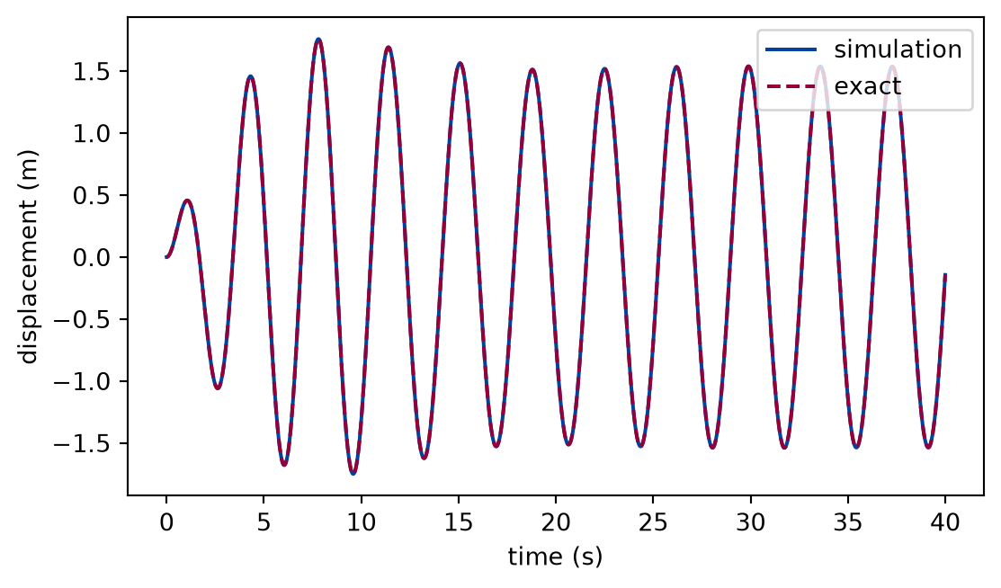
The oscillator of the examples has one kilogram on a spring of four newtons per metre, with the drag constant four tenths of a kilogram per second, so that $\omega_0 = 2\,\mathrm{rad/s}$ and $Q = 5$ . The force has the amplitude two newtons. The cell drives it at 1.7 rad/s, below the natural frequency, from rest, simulates forty seconds at two hundred steps per second, and compares with the exact motion, transient included.

mass, k, b, force = 1.0, 4.0, 0.4, 2.0
w0 = natural_frequency(mass, k)
q = quality_factor(mass, k, b)
gamma = damping_rate(mass, b)
start = State(t=0.0, x=[0.0], v=[0.0])

src/pbc/mechanics/experiments/resonance.py, lines 37 to 41, read from the repository when this page was built.

def closed_form_check(experiment: Experiment):
    """Forty seconds of the oscillator driven at 1.7 rad/s from rest against
    its exact solution; record the table and return the run, the exact
    motion, the largest difference, and the steady-state amplitude."""
    omega = 1.7  # rad/s
    oscillator = newton(mass, spring(k), linear_drag(b), driving_force(force, omega))
    driven = simulate(start, oscillator, 0.005, 8000, step=rk4_step)
    exact = driven_motion(start, mass, k, b, force, omega, driven.t)
    largest = np.max(np.abs(driven.x - exact.x))
    steady = float(steady_state_amplitude(mass, k, b, force, omega))

    experiment.table(
        "closed-form-check",
        [(np.max(np.abs(driven.x)), steady, largest)],
        columns=[
            ("largest displacement of the run", "m", ".4f"),
            ("steady-state amplitude", "m", ".4f"),
            ("largest difference from the exact motion", "m", ".1e"),
        ],
        caption="The simulated motion of the driven oscillator from rest for forty "
        "seconds against its exact solution, with the transient.",
    )
    return driven, exact, largest, steady

src/pbc/mechanics/experiments/resonance.py, lines 45 to 67, read from the repository when this page was built.

The simulated motion of the driven oscillator from rest for forty seconds against its exact solution, with the transient.
largest displacement of the run (m)	steady-state amplitude (m)	largest difference from the exact motion (m)
1.7593	1.5364	8.2e-10

Numerically verified (one driving frequency, forty seconds, classical Runge-Kutta method at the stated step): The simulated motion of the driven oscillator agrees with the exact solution at every instant, the transient included: the largest difference is 8e-10 m against displacements of about 1.54 m. The largest displacement of the run is 1.76 m against the steady-state amplitude 1.54 m: the free motion, which starts so as to cancel the steady state at the first instant, adds to it for a while as it decays.

def draw_transient(driven, exact) -> Figure:
    """The displacement from rest, simulated and exact."""
    fig, ax = plt.subplots(figsize=(6.4, 3.6))
    ax.plot(
        driven.t,
        driven.x[:, 0],
        color=FIGURE_COLOURS[0],
        linestyle="-",
        label="simulation",
    )
    ax.plot(
        driven.t, exact.x[:, 0], color=FIGURE_COLOURS[1], linestyle="--", label="exact"
    )
    ax.set_xlabel("time (s)")
    ax.set_ylabel("displacement (m)")
    ax.legend(loc="upper right")
    return fig

src/pbc/mechanics/experiments/resonance.py, lines 70 to 86, read from the repository when this page was built.

Plot of displacement against time over forty seconds. A solid curve, the simulation, and a dashed curve, the exact motion, lie on top of each other. The oscillation starts at zero, grows to a larger swing within the first ten seconds with an irregular envelope, and then settles into a steady sinusoid of constant amplitude. — Figure 1: simulated The displacement of the driven oscillator from rest, simulated and exact. The motion starts at zero, swells while the free motion and the steady state add up, and settles into a steady oscillation at the driving frequency with the amplitude of the closed form.

The simulation and the exact curve are indistinguishable at this scale, as the table says. The figure shows what the rest of the lesson must avoid: reading an amplitude off the first swings, where the transient dominates.

The resonance curve

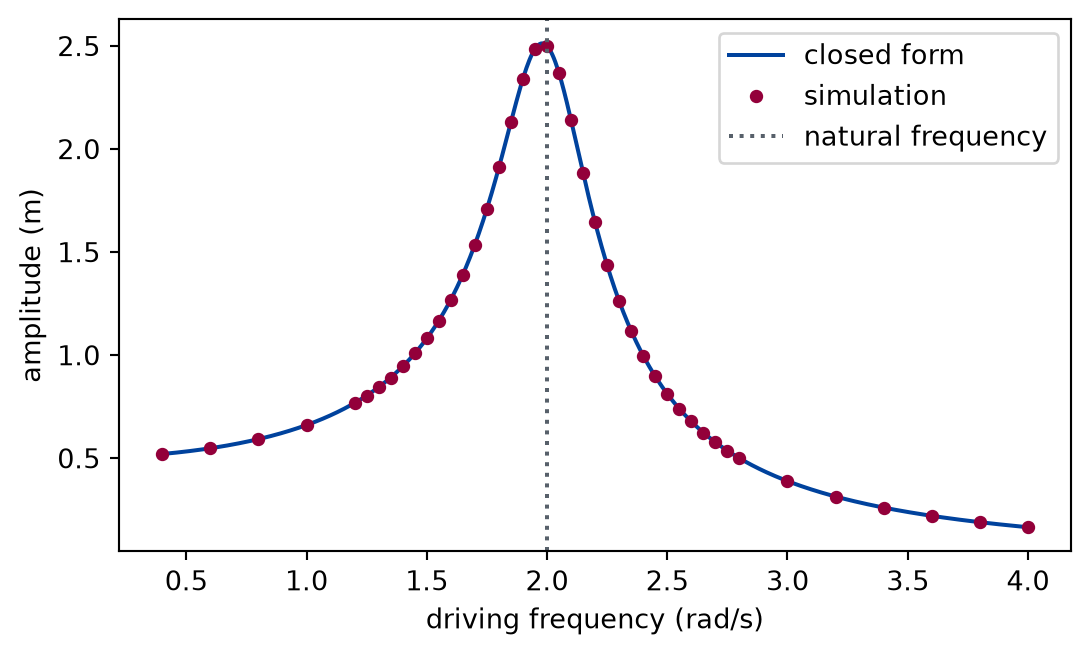
The cell measures the amplitude and the phase at each of forty-three driving frequencies between four tenths and four radians per second, denser around the natural frequency, each time starting from rest, running for eight decay times to let the transient die, and fitting the next ten driving periods. A third of the frequencies are printed.

def resonance_curve(experiment: Experiment):
    """The amplitude and phase lag of the steady state over the driving
    frequency, simulated and closed form; record the table of every third
    frequency."""
    omegas = np.concatenate(
        [
            np.arange(0.4, 1.2, 0.2),
            np.arange(1.2, 2.85, 0.05),
            np.arange(3.0, 4.01, 0.2),
        ]
    )
    measured, phase = measured_resonance_curve(
        mass, k, b, force, omegas, decay_times=8.0
    )
    analytic = steady_state_amplitude(mass, k, b, force, omegas)
    analytic_phase = steady_state_phase(mass, k, b, omegas)

    pick = np.arange(0, len(omegas), 3)
    experiment.table(
        "resonance-curve",
        [
            (omegas[i], analytic[i], measured[i], analytic_phase[i], phase[i])
            for i in pick
        ],
        columns=[
            ("driving frequency", "rad/s", ".2f"),
            ("amplitude, closed form", "m", ".4f"),
            ("amplitude, simulation", "m", ".4f"),
            ("phase lag, closed form", "rad", ".3f"),
            ("phase lag, simulation", "rad", ".3f"),
        ],
        caption="Amplitude and phase lag of the driven oscillator at a third of the "
        "frequencies of the curve: the closed form and the simulation, to four "
        "and three decimals.",
    )
    return omegas, measured, phase, analytic, analytic_phase

src/pbc/mechanics/experiments/resonance.py, lines 89 to 124, read from the repository when this page was built.

Amplitude and phase lag of the driven oscillator at a third of the frequencies of the curve: the closed form and the simulation, to four and three decimals.
driving frequency (rad/s)	amplitude, closed form (m)	amplitude, simulation (m)	phase lag, closed form (rad)	phase lag, simulation (rad)
0.40	0.5204	0.5204	0.042	0.042
1.00	0.6608	0.6608	0.133	0.133
1.30	0.8447	0.8447	0.221	0.221
1.45	1.0080	1.0080	0.297	0.297
1.60	1.2692	1.2692	0.418	0.418
1.75	1.7094	1.7094	0.641	0.641
1.90	2.3413	2.3413	1.097	1.097
2.05	2.3679	2.3680	1.813	1.813
2.20	1.6440	1.6440	2.333	2.333
2.35	1.1178	1.1178	2.588	2.588
2.50	0.8123	0.8123	2.723	2.723
2.65	0.6244	0.6244	2.804	2.804
2.80	0.5000	0.5000	2.858	2.858
3.40	0.2604	0.2604	2.964	2.964
4.00	0.1652	0.1652	3.009	3.009

Numerically verified (forty-three frequencies, classical Runge-Kutta method, amplitude read after eight decay times): The simulated resonance curve agrees with the analytic amplitude at every frequency: the largest relative difference of the amplitude is 4e-05 over all of them, and the largest difference of the phase is 3e-05 rad. The delay passes through a quarter of a turn, 1.571 rad, at the natural frequency, as derived.

def draw_resonance_curve(omegas, measured) -> Figure:
    """The resonance curve, closed form and simulated."""
    dense = np.linspace(0.4, 4.0, 600)
    fig, ax = plt.subplots(figsize=(6.4, 3.6))
    ax.plot(
        dense,
        steady_state_amplitude(mass, k, b, force, dense),
        color=FIGURE_COLOURS[0],
        linestyle="-",
        label="closed form",
    )
    ax.plot(
        omegas,
        measured,
        color=FIGURE_COLOURS[1],
        marker="o",
        linestyle="",
        markersize=4,
        label="simulation",
    )
    ax.axvline(w0, color="#57606a", linestyle=":", label="natural frequency")
    ax.set_xlabel("driving frequency (rad/s)")
    ax.set_ylabel("amplitude (m)")
    ax.legend(loc="upper right")
    return fig

src/pbc/mechanics/experiments/resonance.py, lines 127 to 151, read from the repository when this page was built.

Plot of amplitude in metres against driving frequency in radians per second. A solid smooth line rises from a low value on the left to a sharp peak near the middle, then falls to small values on the right. Round markers from the simulation lie on the line at every frequency. A vertical dotted line marks the natural frequency, just to the right of the peak. — Figure 2: simulated The resonance curve of the driven oscillator: the amplitude of the steady state against the driving frequency. The markers are the simulation, the line is the closed form; they agree. The curve rises from the static displacement, peaks a little below the natural frequency, and falls away.

The figure is the table in full: the markers are the simulation at all frequencies, the line the closed form. The peak is within a few per cent of the natural frequency and its height is far above the static displacement.

Peak, width, and quality factor

The peak height, position, and width are read from the measured curve and compared with the formulas of the explanation: the exact peak of the closed form, and the approximations for weak damping. The position and the height of the maximum are those of the sample with the largest amplitude, so they are accurate to the spacing of the samples.

def peak_and_width(experiment: Experiment, omegas, measured):
    """The peak and the width of the resonance, closed form and read from the
    simulated curve; record the table."""
    width = half_power_width(omegas, measured)
    w_peak = peak_frequency(mass, k, b)
    exact_peak = float(steady_state_amplitude(mass, k, b, force, w_peak))
    rows = [
        ("peak frequency", "rad/s", w_peak, omegas[np.argmax(measured)]),
        ("peak height", "m", exact_peak, np.max(measured)),
        ("full width at half power", "rad/s", b / mass, width),
        ("quality factor", "", q, w0 / width),
    ]
    experiment.table(
        "peak-and-width",
        rows,
        columns=[
            ("quantity", "", ""),
            ("unit", "", ""),
            ("closed form", "", ".3f"),
            ("from the simulated curve", "", ".3f"),
        ],
        caption="The peak frequency, height, width at half power, and quality "
        "factor of the resonance: the closed forms and the values read from the "
        "simulated curve, to three decimals.",
    )
    return width, w_peak, exact_peak

src/pbc/mechanics/experiments/resonance.py, lines 154 to 179, read from the repository when this page was built.

The peak frequency, height, width at half power, and quality factor of the resonance: the closed forms and the values read from the simulated curve, to three decimals.
quantity	unit	closed form	from the simulated curve
peak frequency	rad/s	1.980	2.000
peak height	m	2.513	2.500
full width at half power	rad/s	0.400	0.411
quality factor		5.000	4.865

The peak lies at 1.980 rad/s, below the natural frequency 2.000 rad/s, and the samples have the maximum at 2.00 rad/s. The weak-damping height $Q F_0/k$ , 2.500 m, is within 0.5% of the exact peak. The width at half power is 0.411 rad/s against $b/m =$ 0.400 rad/s, and the quality factor read from it, 4.86, against 5.00 from the parameters, a difference of 3%. Numerically verified (one oscillator, the samples of the curve above): The quality factor read from the width of the simulated curve is the one that the parameters give, to the accuracy of the sampling of the curve.

How long to settle

The transient is the free motion, which falls as $e^{-\gamma t}$ . The cell takes the exact motion for the drive at the natural frequency from rest, subtracts the steady state, and finds the time after which what is left stays below one per cent of the steady-state amplitude, for the oscillator above and for one with a quarter of the damping.

def settling(experiment: Experiment) -> list:
    """The time the transient takes to stay below one per cent of the steady
    state, for two quality factors; record the table and return its rows."""
    rows = []
    for factor in (1.0, 0.25):
        b_case = b * factor
        amplitude = float(steady_state_amplitude(mass, k, b_case, force, w0))
        delta = float(steady_state_phase(mass, k, b_case, w0))
        t = np.linspace(0.0, 400.0, 400001)
        motion = driven_motion(start, mass, k, b_case, force, w0, t)
        leftover = np.abs(motion.x[:, 0] - amplitude * np.cos(w0 * t - delta))
        settled = t[np.where(leftover > 0.01 * amplitude)[0][-1]]
        rows.append(
            (quality_factor(mass, k, b_case), settled, 1.0 / damping_rate(mass, b_case))
        )

    experiment.table(
        "settling",
        rows,
        columns=[
            ("quality factor", "", ".1f"),
            ("time to settle to one per cent", "s", ".1f"),
            ("decay time 1/gamma", "s", ".1f"),
        ],
        caption="The time after which the transient stays below one per cent of the "
        "steady-state amplitude, for two quality factors, with the decay time of "
        "the free motion.",
    )
    return rows

src/pbc/mechanics/experiments/resonance.py, lines 182 to 210, read from the repository when this page was built.

The time after which the transient stays below one per cent of the steady-state amplitude, for two quality factors, with the decay time of the free motion.
quality factor	time to settle to one per cent (s)	decay time 1/gamma (s)
5.0	23.0	5.0
20.0	92.0	20.0

The settling time is a few decay times, 4.6 and 4.6 of them, and it grows with $Q$ : the oscillator with 4 times the quality factor takes 4.0 times as long. The sharpness of the resonance and the time it takes to reach it are bought together.

Limits

The oscillator is linear and the amplitude of the drive does not change the shape of the curve; the curve of a real spring that stiffens at large stretch would lean to one side. The lesson has no such system, and the validation is of the linear model only.
The validation is of the program against the closed form of the same model, not against a measurement. A measured resonance would have noise, a background, and a damping that is not linear; the pendulum and accelerometer lab of the measured-data strand returns to it.
The peak height and position are read at the sampling of the frequencies, so they are accurate to the spacing of the samples, and the width by linear interpolation between them.
The formula for the width, $b/m$ , and the equality of $Q$ with the ratio of the peak frequency to the width are approximations for weak damping; for strong damping they differ, and a peak may not exist.
The closed form of the transient is for damping below the critical value. The steady state, and the simulation, do not depend on that.
The settling time is read for two cases and for a bound of one per cent; it is of the order of the decay time, not a precise multiple.

Self-check. A system is driven at exactly its natural frequency by a force of constant amplitude. Does the amplitude grow without limit? Say what sets the size of the steady state, and what would change if the damping were zero.

With scripts, you can record in this browser that you answered this question.

Solution to the self-check

With damping the amplitude stops growing. The motion settles at the amplitude at which the energy the force puts in during a swing equals what the drag takes out: the steady state of the lesson, whose height is the static displacement times $Q$ . The longer the system rings, the larger the quality factor, the larger the peak, and the longer it takes to reach it. Without damping the closed form has no finite value at the natural frequency, the denominator vanishing, and the amplitude of the motion from rest grows in proportion to the time: nothing takes the energy out. A real system never has zero damping, and a real spring stops being linear long before the amplitude is large, which limits the growth in another way.

Exercises

Exercise 1. Ring-down. Release the oscillator of the examples from one metre at rest with no force and let it ring. Read the quality factor from the decay of the successive peaks, and compare it with $\sqrt{k m}/b$ .

Hint 1 of 2 for exercise 1

The logarithm of the peak heights falls along a straight line whose slope is minus the damping rate.

Hint 2 of 2 for exercise 1

Take the peaks as the local maxima of the displacement, and fit a line to the logarithm of their heights against their times.

Solution to exercise 1

def free_decay(experiment: Experiment) -> float:
    """Exercise 1: the decay rate and the quality factor from the peaks of
    the free motion; record the table and return the decay rate, in 1/s."""
    free = simulate(
        State(0.0, [1.0], [0.0]),
        newton(mass, spring(k), linear_drag(b)),
        0.005,
        8000,
        step=rk4_step,
    )
    x = free.x[:, 0]
    peaks = np.where((x[1:-1] > x[:-2]) & (x[1:-1] >= x[2:]) & (x[1:-1] > 0))[0] + 1
    slope, _ = np.polyfit(free.t[peaks], np.log(x[peaks]), 1)
    rate = -slope
    q_free = w0 / (2.0 * rate)

    experiment.table(
        "free-decay",
        [(rate, gamma, q_free, q)],
        columns=[
            ("decay rate from the peaks", "1/s", ".4f"),
            ("b / 2m", "1/s", ".4f"),
            ("Q from the decay", "", ".3f"),
            ("Q from the parameters", "", ".3f"),
        ],
        caption="The decay rate and the quality factor read from the peaks of the "
        "free motion and from the parameters, to the precision shown.",
    )
    return rate

src/pbc/mechanics/experiments/resonance.py, lines 213 to 241, read from the repository when this page was built.

The decay rate and the quality factor read from the peaks of the free motion and from the parameters, to the precision shown.
decay rate from the peaks (1/s)	b / 2m (1/s)	Q from the decay	Q from the parameters
0.2000	0.2000	5.000	5.000

The decay rate from the peaks is the damping rate $b/2m$ , and the quality factor follows from it; they agree to a relative 4e-05, the difference being that the peaks are read at the sampled instants, a step apart, and not at the true maxima.

Exercise 2. Halving the peak. By what factor must the damping constant rise to halve the height of the resonance peak? Predict it from the closed form, then confirm it with the program.

Hint 1 of 1 for exercise 2

For weak damping the peak height is the force amplitude divided by the product of the damping constant and the natural frequency.

Solution to exercise 2

def doubled_damping(experiment: Experiment) -> list:
    """Exercise 2: the peak height for the damping constant and for twice it;
    record the table and return the heights, in m."""
    heights = []
    for factor in (1.0, 2.0):
        b_case = b * factor
        top = steady_state_amplitude(
            mass, k, b_case, force, peak_frequency(mass, k, b_case)
        )
        heights.append(float(top))

    experiment.table(
        "doubled-damping",
        [(1.0, heights[0], 1.0), (2.0, heights[1], heights[1] / heights[0])],
        columns=[
            ("damping, in units of b", "", ".1f"),
            ("peak height", "m", ".4f"),
            ("relative to the first", "", ".3f"),
        ],
        caption="The peak height of the resonance curve for the damping constant and "
        "for twice it, to four decimals, with the ratio.",
    )
    return heights

src/pbc/mechanics/experiments/resonance.py, lines 244 to 266, read from the repository when this page was built.

The peak height of the resonance curve for the damping constant and for twice it, to four decimals, with the ratio.
damping, in units of b	peak height (m)	relative to the first
1.0	2.5126	1.000
2.0	1.2758	0.508

The peak height is inversely proportional to the damping for weak damping, so the damping must double to halve the peak; the table gives 0.508 for the exact peak, slightly above one half because the peak frequency also moves. Doubling the damping also doubles the width of the resonance and halves the time to settle: the same quality factor controls all three.

Run this experiment

This page was built from commit 6417e2ff90258bd2d2ba21d217eb7666fd24f680 of the repository.

In a clone at that commit, with the project’s Python packages installed, this command runs the experiment of this page:

uv run --locked --no-dev python -m pbc.mechanics.experiments.resonance results

Files, tests, and every command

The files behind it:

site/lessons/mechanics/16-resonance/index.qmd: this page, with every code cell.
src/pbc/mechanics/dynamics.py: code the experiment runs.
src/pbc/mechanics/integrators.py: code the experiment runs.
src/pbc/mechanics/oscillator.py: code the experiment runs.
src/pbc/mechanics/drag.py: code the experiment runs.
src/pbc/mechanics/resonance.py: code the experiment runs.
src/pbc/mechanics/experiments/resonance.py: code the experiment runs.
src/pbc/experiment.py: code the experiment runs.
tests/unit/test_integrators.py: tests of that code.
tests/unit/test_oscillator.py: tests of that code.
tests/unit/test_drag.py: tests of that code.
tests/unit/test_resonance.py: tests of that code.
tests/unit/test_resonance_experiment.py: tests of that code.

With Git and uv installed (see the setup page), run:

git clone https://github.com/taspinar/physics-by-construction.git
cd physics-by-construction
git checkout 6417e2ff90258bd2d2ba21d217eb7666fd24f680
uv sync --locked --no-dev
uv run --locked --no-dev python -m pbc.mechanics.experiments.resonance results

The experiment writes every figure of this page into results/, as <label>.png, and every number and table of the page, as the page shows it, into results/results.json. Its numbers match this page to the digits shown, and its figure files are the ones the page shows; digits beyond those can differ between machines, because floating-point libraries differ. Change the code of the experiment and run it again to see what changes.