Kinetic theory of gases

Why a gas of colliding particles settles into the Maxwell distribution of speeds, and a check of the simulated gas of the first lesson against the analytic distribution at the temperature the simulation reached.

Course

Thermodynamics and statistical physics, lesson 3 of 4

Slot

T2, Kinetic theory of gases

Methods

Simulation

Difficulty

Intermediate, level 2 of 3

What you’ll learn

Derive the Maxwell distribution of speeds from the independence and the isotropy of the velocity components
Define the temperature of a gas from its mean kinetic energy
Check the speeds of a simulated gas against the analytic distribution at its own temperature, within a stated tolerance

Prerequisites

Particles in a box.

Before you begin

Probability: the Gaussian distribution, the distribution function of a random variable, and its quantiles
Statistics: the mean, the standard deviation, and the standard error of a mean
Calculus: integrating a Gaussian, and changing to polar coordinates

Related

Random walks and diffusion

Previous

Random walks and diffusion

Next

Entropy from ensembles

With scripts, this page keeps a record in your browser of whether you completed the lesson. Nothing is stored without them.

With scripts, this place suggests what to do next, with the reason, from the progress saved in your browser. Without them, follow the learning path.

The molecules of the air in a room move at hundreds of metres per second, and each of them changes its velocity billions of times a second in collisions with the others. No molecule keeps its speed, yet the fraction of molecules that move faster than some value is steady, and the value that marks the fastest tenth of them depends on one number, the temperature. Where does that distribution come from, and why does only the temperature appear in it?

The gas lesson built a gas of colliding discs and showed that its speeds follow the Maxwell distribution, by one moment ratio. This lesson takes that gas as it is, from pbc.abm.gas, and asks the question in the other order. First it derives what the distribution has to be, from two properties of the collisions. Then it measures the whole curve, not one moment, at the temperature the simulated gas has reached, and compares it with the derived curve at several points. The checks are numerical checks of a model against a theory, with the tolerance of the gas lesson. No real gas is measured here.

Assumptions

The gas of the first lesson. Two-dimensional identical hard discs, elastic collisions, perfectly reflecting walls, a dilute gas, and a time step that resolves a collision. The assumptions of that lesson hold here unchanged, and the numbers below are those of that gas: the three-dimensional curve is different.
The velocity components are independent and the gas is isotropic. The derivation needs that the probability of a velocity depends only on its length, not on a direction, and that the two components do not influence each other. A gas with a bulk flow, or one held in a field that favours a direction, breaks isotropy. The simulation removes the mean velocity at the start for this reason.
The gas has relaxed. The distribution is the end of the collisions, not their start. The measurement begins after the relaxation time of the gas lesson, and a measurement taken earlier would see the start, a narrow band of speeds.
The temperature is the mean kinetic energy. The program defines $k_BT$ as the mean kinetic energy of a disc, $\tfrac12 m\langle v^2\rangle$ , which is the temperature of a two-dimensional gas when each direction holds $\tfrac12k_BT$ . The comparison therefore uses a distribution at the energy that the same speeds give, not at an independently measured temperature, and the check tests the shape, not the absolute scale.
The runs are independent, the snapshots are not. The speeds of one run at successive snapshots, and the discs within a snapshot, are correlated. The standard error is taken from the spread between runs with different seeds, never from the number of discs or snapshots.
Randomness is seeded. A run is a function of its seed, so the page is the same at every build.

Explanation

What the distribution has to be

Take the probability density of the velocity $(v_x, v_y)$ of one disc in the relaxed gas. Two things are known about it. The plane has no preferred direction, so the density depends only on the speed, $f(v_x, v_y) = g(v^2)$ . And the two components are independent, so it is also a product, $f = h(v_x)\,h(v_y)$ . A function of $v_x^2 + v_y^2$ that is also a product of a function of $v_x$ and a function of $v_y$ must be an exponential of the square: taking the logarithm, $\ln g(v_x^2 + v_y^2) = \ln h(v_x) + \ln h(v_y)$ , and putting $v_y = 0$ and then differentiating shows that $\ln h$ is a constant minus a constant times $v_x^2$ . So each component is Gaussian with mean zero,

$h(v_x) \propto \exp\!\left(-\frac{m v_x^2}{2k_BT}\right),$

where the constant in the exponent is the definition of the temperature: $\langle \tfrac12 m v_x^2\rangle = \tfrac12 k_BT$ for each of the two directions. The argument says what the form must be if the collisions give the gas the two properties. It does not show that they do; that is what the simulation tests.

The distribution of speeds

In polar coordinates the area element is $v\,\mathrm dv\,\mathrm d\theta$ , and the density depends only on $v$ , so integrating over the angle gives the density of the speed,

$f(v) = \frac{m v}{k_BT}\exp\!\left(-\frac{m v^2}{2k_BT}\right).$

A check against measured speeds is easier with the distribution function, the probability that a disc is slower than $v$ , which the integral of $f$ gives in closed form,

$F(v) = 1 - \exp\!\left(-\frac{m v^2}{2k_BT}\right).$

Its inverse is the speed below which a fraction $p$ of the discs lie, $v_p = \sqrt{-2k_BT\ln(1 - p)/m}$ . Two other numbers follow from the density: the speed at which it peaks, $\sqrt{k_BT/m}$ , and the mean speed $\langle v\rangle = \sqrt{\pi k_BT/(2m)}$ . The mean is larger than the peak because the density has a long tail towards high speeds.

The check

The simulated gas has a temperature, $k_BT = \tfrac12 m\langle v^2\rangle$ , from its own speeds. The check takes that temperature, computes the speeds $v_p$ below which the distribution says the fractions $p = 0.1, 0.25, 0.5, 0.75, 0.9$ lie, and counts the fraction of the gas that is really below each. If the distribution is right, the counted fraction is $p$ . The count is made in each independent run, and the mean over the runs is compared with $p$ in units of its standard error, with the tolerance of the gas lesson: agreement within $4$ standard errors, a chosen tolerance, not a law. With six runs the standard error is itself uncertain, so chance alone exceeds four standard errors in about one case in a hundred at one point, and a failure at several points is a reason to look at the model, not a proof against it.

Code

The analytic distribution is pbc.thermodynamics.kinetic: the distribution function, its inverse, and the two characteristic speeds. The gas is the one of the first lesson, run by pbc.abm.gas.measure, which this lesson calls without change.

def speed_cdf(speed: Array, kt: float, mass: float) -> Array:
    """The probability 1 - exp(-m v² / (2 k_B T)) that a disc is slower than
    ``speed`` (m/s)."""
    v = np.asarray(speed, dtype=np.float64)
    return 1.0 - np.exp(-mass * v**2 / (2.0 * kt))

src/pbc/thermodynamics/kinetic.py, lines 16 to 20, read from the repository when this page was built.

def speed_quantile(probability: Array, kt: float, mass: float) -> Array:
    """The speed (m/s) that a fraction ``probability`` of the discs is slower
    than: the inverse of ``speed_cdf``, sqrt(-2 k_B T ln(1 - p) / m)."""
    p = np.asarray(probability, dtype=np.float64)
    return np.sqrt(-2.0 * kt * np.log1p(-p) / mass)

src/pbc/thermodynamics/kinetic.py, lines 23 to 27, read from the repository when this page was built.

The measured side is the fraction of speeds below a threshold, the empirical distribution function.

def fractions_below(speeds: Array, thresholds: Array) -> Array:
    """The fraction of ``speeds`` below each of the ``thresholds``: the
    empirical distribution function at those speeds."""
    s = np.sort(np.asarray(speeds, dtype=np.float64).ravel())
    return np.searchsorted(s, np.asarray(thresholds), side="left") / s.size

src/pbc/thermodynamics/kinetic.py, lines 40 to 44, read from the repository when this page was built.

Worked examples

The speeds of the relaxed gas at the quantiles of the model

Six runs of the gas of the first lesson, each from its own seed, relaxed and then measured. For each run the quantile speeds are computed at that run’s temperature.

MASS = 1.0  # the mass of a disc in pbc.abm.gas, kg
SEEDS = range(6)
PROBABILITIES = np.array([0.1, 0.25, 0.5, 0.75, 0.9])

src/pbc/thermodynamics/experiments/kinetic_theory_of_gases.py, lines 29 to 31, read from the repository when this page was built.

def quantile_check(experiment: Experiment):
    """Six runs of the gas, and the fraction of their speeds below the
    quantile speeds of the Maxwell distribution; record the table and return
    the measurements and the distances in standard errors."""
    measurements = [measure(seed) for seed in SEEDS]
    fractions = np.array(
        [
            fractions_below(m.speeds, speed_quantile(PROBABILITIES, m.kt, MASS))
            for m in measurements
        ]
    )
    means = fractions.mean(axis=0)
    errors = fractions.std(axis=0, ddof=1) / np.sqrt(len(measurements))
    distances = np.abs(means - PROBABILITIES) / errors

    experiment.table(
        "quantile-check",
        list(zip(PROBABILITIES, means, errors, distances, strict=True)),
        [
            ("predicted fraction", "", ".2f"),
            ("measured fraction", "", ".3f"),
            ("standard error", "", ".3f"),
            ("difference", "standard errors", ".1f"),
        ],
        "The fraction of the speeds below the quantile speed of the Maxwell "
        "distribution at the temperature of each run, averaged over six runs, at "
        "five predicted fractions.",
    )
    return measurements, distances

src/pbc/thermodynamics/experiments/kinetic_theory_of_gases.py, lines 35 to 63, read from the repository when this page was built.

The fraction of the speeds below the quantile speed of the Maxwell distribution at the temperature of each run, averaged over six runs, at five predicted fractions.
predicted fraction	measured fraction	standard error	difference (standard errors)
0.10	0.095	0.002	2.2
0.25	0.241	0.004	2.4
0.50	0.497	0.004	0.9
0.75	0.746	0.003	1.4
0.90	0.900	0.002	0.1

Numerically verified (a dilute gas of hard discs in two dimensions, six seeds, five quantiles, four standard errors): The speeds of the relaxed gas follow the Maxwell distribution at its own temperature: the measured fraction below each of five quantile speeds agrees with the predicted fraction within four standard errors. The largest difference is 2.4 standard errors, over five points of the curve, from the tenth to the ninetieth percentile.

A wrong temperature is seen

A check that cannot fail is worth nothing. Take the same speeds and compare them with the distribution at a temperature that is ten per cent too high, the kind of error a mistaken definition of the temperature would make.

def wrong_temperature(experiment: Experiment, measurements):
    """The same comparison at a temperature ten per cent too high; record the
    table and return the distances in standard errors."""
    scale = 1.1
    wrong = np.array(
        [
            fractions_below(m.speeds, speed_quantile(PROBABILITIES, scale * m.kt, MASS))
            for m in measurements
        ]
    )
    wrong_means = wrong.mean(axis=0)
    wrong_errors = wrong.std(axis=0, ddof=1) / np.sqrt(len(measurements))
    wrong_distances = np.abs(wrong_means - PROBABILITIES) / wrong_errors

    experiment.table(
        "wrong-temperature",
        list(zip(PROBABILITIES, wrong_means, wrong_distances, strict=True)),
        [
            ("predicted fraction", "", ".2f"),
            ("measured fraction", "", ".3f"),
            ("difference", "standard errors", ".1f"),
        ],
        "The same comparison against the distribution at a temperature ten per "
        "cent too high.",
    )
    return wrong_distances

src/pbc/thermodynamics/experiments/kinetic_theory_of_gases.py, lines 66 to 91, read from the repository when this page was built.

The same comparison against the distribution at a temperature ten per cent too high.
predicted fraction	measured fraction	difference (standard errors)
0.10	0.104	2.1
0.25	0.263	3.5
0.50	0.529	8.8
0.75	0.779	11.6
0.90	0.922	20.8

The wrong curve fails at 3 of the five points, by up to 21 standard errors, so the check has the power to tell a ten per cent error in the temperature from the right value. A smaller error may not be seen.

The curve and the mean speed

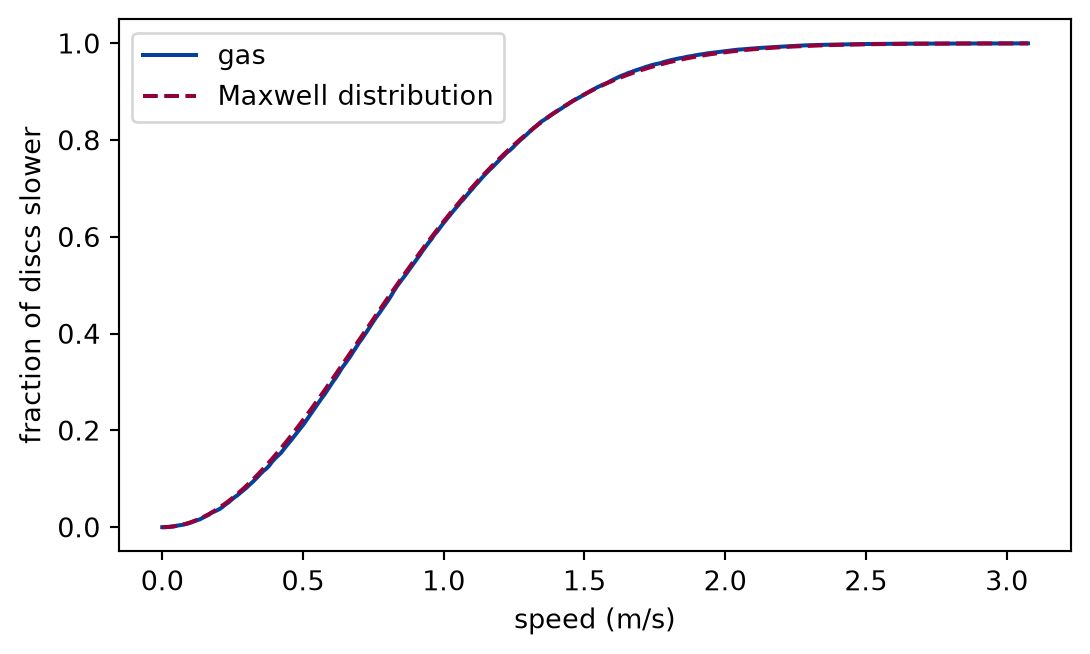
def draw_speed_distribution(measurements) -> Figure:
    """The pooled speeds of the six runs against the Maxwell distribution."""
    pooled = np.concatenate([m.speeds.ravel() for m in measurements])
    kt = float(np.mean([m.kt for m in measurements]))
    v = np.linspace(0.0, pooled.max(), 300)

    fig, ax = plt.subplots(figsize=(6.4, 3.6))
    ax.plot(v, fractions_below(pooled, v), color="#00429d", label="gas")
    ax.plot(
        v,
        speed_cdf(v, kt, MASS),
        color="#93003a",
        linestyle="--",
        label="Maxwell distribution",
    )
    ax.set_xlabel("speed (m/s)")
    ax.set_ylabel("fraction of discs slower")
    ax.legend()
    return fig

src/pbc/thermodynamics/experiments/kinetic_theory_of_gases.py, lines 94 to 112, read from the repository when this page was built.

Line plot of the fraction of discs slower than a speed against the speed in metres per second. A solid curve of the measured speeds rises from zero in an S shape towards one, and a dashed curve of the Maxwell distribution function lies close along it. — Figure 1: simulated The distribution function of the measured speeds follows the Maxwell distribution function at the temperature of the gas; the two curves are close all along, and the checks above say how close.

The pooled speeds of the six runs are used for the picture only, which the fifth assumption allows for a picture and not for a standard error. The figure and the table agree: the gas follows the curve.

def mean_speed_check(experiment: Experiment, measurements):
    """The two characteristic speeds at the mean temperature, and the ratio
    of the measured mean speed to the predicted one; record the table."""
    kt = float(np.mean([m.kt for m in measurements]))
    ratios = np.array(
        [np.mean(m.speeds) / mean_speed(m.kt, MASS) for m in measurements]
    )
    ratio_mean, ratio_error = mean_and_error(ratios)

    experiment.table(
        "mean-speed-check",
        [
            (
                mean_speed(kt, MASS),
                most_probable_speed(kt, MASS),
                ratio_mean,
                ratio_error,
                abs(ratio_mean - 1.0) / ratio_error,
            )
        ],
        [
            ("mean speed", "m/s", ".3f"),
            ("most probable speed", "m/s", ".3f"),
            ("measured mean / predicted mean", "", ".4f"),
            ("standard error", "", ".4f"),
            ("difference", "standard errors", ".1f"),
        ],
        "The two characteristic speeds at the mean temperature of the six runs, "
        "and the ratio of the measured mean speed to the predicted one.",
    )
    return ratio_mean, ratio_error

src/pbc/thermodynamics/experiments/kinetic_theory_of_gases.py, lines 115 to 145, read from the repository when this page was built.

The two characteristic speeds at the mean temperature of the six runs, and the ratio of the measured mean speed to the predicted one.
mean speed (m/s)	most probable speed (m/s)	measured mean / predicted mean	standard error	difference (standard errors)
0.886	0.707	1.0043	0.0017	2.5

The mean speed is larger than the most probable speed, as the long tail of the density requires, and the measured mean agrees with the predicted one: their ratio is 1.0043, 2.5 standard errors from one.

Limits

A model checked against a theory, not against a gas. The data are simulated, and the result says that the model produces the distribution that the derivation predicts. It says nothing about air; no claim of this lesson is experimentally supported.
The temperature is not independent. The same speeds give the temperature and are compared with the curve at that temperature, so the comparison tests the shape of the distribution at a scale it fixes itself. The absolute scale of the distribution is a definition here, and a check against a thermometer would be a different test.
Five points and a tolerance. The quantiles sample the curve at five places, and a model wrong by less than four standard errors passes. The test of a wrong temperature shows the size of error that is seen.
Two dimensions. The curve is that of a plane. In three dimensions the speed density has a factor $v^2$ and the mean speed another constant; the method of the check would be the same.
A dilute, simple gas. Only hard elastic discs at a small packing fraction are modelled: no internal motion, no attraction, no dense liquid.

Self-check. The derivation says that independence of the components and isotropy force a Gaussian. Why is it then not enough to show that the simulated gas has zero mean velocity?

With scripts, you can record in this browser that you answered this question.

Solution to the self-check

A zero mean velocity says only that the first moment vanishes, and many distributions have it. The derivation needs the full density to depend on the speed alone and to factor into the two components; the check of the quantile fractions tests the whole shape of the speed distribution, which is where a gas that is isotropic and independent differs from one that is merely at rest on average.

Exercises

Exercise 1. A hotter gas. Start the gas at twice the speed and measure one seed. By what factor does the temperature change, and does the fraction below the median speed of the model stay at one half?

Hint 1 of 1 for exercise 1

The temperature is the mean kinetic energy.

Solution to exercise 1

The kinetic energy is proportional to the square of the speed, so the temperature rises by a factor of four. The shape of the distribution at the new temperature is the same curve in units of $\sqrt{k_BT/m}$ .

def hot_gas(experiment: Experiment, measurements) -> None:
    """Exercise 1: a gas started twice as fast; record the table."""
    hot = measure(0, speed=2.0 * SPEED)
    cold = measurements[0]
    median = speed_quantile(np.array([0.5]), hot.kt, MASS)
    experiment.table(
        "hot-gas",
        [(hot.kt / cold.kt, fractions_below(hot.speeds, median)[0])],
        [
            ("temperature ratio", "", ".2f"),
            ("fraction below the predicted median", "", ".3f"),
        ],
        "The temperature of the hot gas in units of that of the first gas, and the "
        "fraction of its speeds below the median of the model at its own "
        "temperature.",
    )

src/pbc/thermodynamics/experiments/kinetic_theory_of_gases.py, lines 148 to 163, read from the repository when this page was built.

The temperature of the hot gas in units of that of the first gas, and the fraction of its speeds below the median of the model at its own temperature.
temperature ratio	fraction below the predicted median
4.00	0.506

One seed is one run, so the fraction differs from one half by about the spread between runs.

Exercise 2. Fewer collisions. Measure one seed without relaxing it. What does the distribution look like at the quantiles?

Solution to exercise 2

Without relaxation the speeds are still the narrow band of the start, so the fractions below the quantile speeds are far from the predicted ones.

def before_relaxation(experiment: Experiment) -> None:
    """Exercise 2: a gas measured during its first half second; record the
    table."""
    start = measure(0, relax=0.0, duration=0.5)
    raw = fractions_below(start.speeds, speed_quantile(PROBABILITIES, start.kt, MASS))
    experiment.table(
        "before-relaxation",
        list(zip(PROBABILITIES, raw, strict=True)),
        [("predicted fraction", "", ".2f"), ("measured fraction", "", ".3f")],
        "The fraction of the speeds below each quantile of the model, for a gas "
        "measured during its first half second.",
    )

src/pbc/thermodynamics/experiments/kinetic_theory_of_gases.py, lines 166 to 177, read from the repository when this page was built.

The fraction of the speeds below each quantile of the model, for a gas measured during its first half second.
predicted fraction	measured fraction
0.10	0.034
0.25	0.114
0.50	0.301
0.75	0.802
0.90	0.957

Run this experiment

This page was built from commit 6417e2ff90258bd2d2ba21d217eb7666fd24f680 of the repository.

In a clone at that commit, with the project’s Python packages installed, this command runs the experiment of this page:

uv run --locked --no-dev python -m pbc.thermodynamics.experiments.kinetic_theory_of_gases results

Files, tests, and every command

The files behind it:

site/lessons/thermodynamics/02-kinetic-theory-of-gases/index.qmd: this page, with every code cell.
src/pbc/thermodynamics/kinetic.py: code the experiment runs.
src/pbc/abm/gas.py: code the experiment runs.
src/pbc/thermodynamics/experiments/kinetic_theory_of_gases.py: code the experiment runs.
src/pbc/experiment.py: code the experiment runs.
tests/unit/test_thermodynamics.py: tests of that code.
tests/unit/test_gas.py: tests of that code.
tests/unit/test_kinetic_theory_of_gases_experiment.py: tests of that code.

With Git and uv installed (see the setup page), run:

git clone https://github.com/taspinar/physics-by-construction.git
cd physics-by-construction
git checkout 6417e2ff90258bd2d2ba21d217eb7666fd24f680
uv sync --locked --no-dev
uv run --locked --no-dev python -m pbc.thermodynamics.experiments.kinetic_theory_of_gases results

The experiment writes every figure of this page into results/, as <label>.png, and every number and table of the page, as the page shows it, into results/results.json. Its numbers match this page to the digits shown, and its figure files are the ones the page shows; digits beyond those can differ between machines, because floating-point libraries differ. Change the code of the experiment and run it again to see what changes.