Entropy from ensembles

Entropy as the logarithm of a count of microstates, grown from an ensemble of boxes of particles, checked against a case with a closed form, and the limits of what an estimate of an entropy can tell.

Course

Thermodynamics and statistical physics, lesson 4 of 4

Slot

T3, Entropy and thermodynamic equilibrium

Methods

Simulation

Difficulty

Intermediate, level 2 of 3

What you’ll learn

Count the microstates of a macrostate and write the entropy as the logarithm of the count
Evolve an ensemble of boxes and estimate its entropy from the observed frequencies
Check the entropy of the ensemble against its value at equilibrium, and say what an estimate from a finite ensemble can and cannot show

Prerequisites

Random walks and diffusion.

Before you begin

Probability: probabilities of independent events, and the binomial distribution
Logarithms: the natural logarithm of a product, and of a factorial for large numbers
Statistics: the mean, the standard deviation, and the standard error of a mean

Related

Kinetic theory of gases

Previous

Kinetic theory of gases

Next

The wave equation

With scripts, this page keeps a record in your browser of whether you completed the lesson. Nothing is stored without them.

With scripts, this place suggests what to do next, with the reason, from the progress saved in your browser. Without them, follow the learning path.

Gas released into one half of a box fills the whole box and never returns to the half by itself, although every collision that spread it could run backwards without breaking a law of motion. What makes the spreading a one-way street? And what does it mean that entropy, the quantity that tells the direction, goes up?

The answer of statistical physics is a count. A configuration of the gas in detail is a microstate. Only a few numbers, such as how many particles are in the left half, are visible in a measurement, and many microstates belong to each such macrostate. The entropy is the logarithm of that count, and the spreading is the gas moving to the macrostates that have the most microstates. This lesson builds the smallest model with that structure, two halves and a few distinguishable particles that are shuffled at random, a random walk of the number on the left, as in the diffusion lesson, and computes the entropy of an ensemble of copies of it. There is a case with a closed form: the entropy of the ensemble at equilibrium is the logarithm of the number of all microstates. The measurement is checked against that, and the lesson says where the check stops being informative. The data are simulated, and entropy is in units of the Boltzmann constant.

Assumptions

Distinguishable particles in two halves. The state of the model is which half each of $N$ particles is in. Positions within a half and velocities are not modelled. Real gases have a continuum of microstates and a measure on them, which the count here replaces.
Every microstate of a macrostate is equally likely. The entropy below is the entropy of an ensemble in which this holds within each macrostate. The dynamics keeps it true when the ensemble starts so, and the start does: all particles on the left is one microstate.
The dynamics is a random shuffle. One step chooses a particle uniformly at random and puts it in the left or the right half with probability one half each, wherever it was. This is a model of equilibration, not of Newton’s laws, and it is not reversible in time in the sense that a trajectory of the model can be run backwards with the same probability only on average. A step that always moved the particle to the other half would let the number on the left alternate between even and odd for ever, and the ensemble would never reach equilibrium, so the model avoids it.
Independent boxes. The members of an ensemble do not interact. The entropy estimate treats the boxes as independent draws from one distribution.
Entropy in nats and in units of $k_B$ . $S/k_B = \ln\Omega$ with the natural logarithm; multiply by $k_B$ for joules per kelvin.
Enough boxes. The estimate of an entropy from observed frequencies is biased low when the ensemble is small. The lesson measures the bias, corrects for it to first order, and says when the correction is not enough.
Randomness is seeded. Each run starts from a seed, so a run is a function of its inputs and the page is the same at every build. The standard error comes from independent runs, never from the boxes of one run.

Explanation

Microstates, macrostates, and the entropy of a count

A microstate says, for each of $N$ distinguishable particles, left or right. There are $2^N$ of them. A macrostate says only the number $n$ on the left, and the number of microstates that give it is the binomial coefficient

$\Omega(n) = \binom{N}{n} = \frac{N!}{n!\,(N-n)!}.$

Boltzmann’s entropy of the macrostate is $S = k_B\ln\Omega(n)$ . It is zero when all particles are on the left, $n = N$ , which is one microstate, and largest at $n = N/2$ . For large $N$ Stirling’s approximation $\ln N! \approx N\ln N - N$ gives

$\ln\binom{N}{N/2} \approx N\ln 2 - \tfrac12\ln\frac{\pi N}{2},$

which differs from the exact value by a term that vanishes as $N$ grows. The leading term, $N\ln 2$ , is the logarithm of all $2^N$ microstates: at the top the biggest macrostate holds almost all of them, on a logarithmic scale.

The entropy of an ensemble

A single box has a macrostate, not a probability. An ensemble is many copies of the box, and gives the probability $p_n$ that a box has $n$ particles on the left. If every microstate of a macrostate is equally likely, the probability of one microstate with $n$ on the left is $p_n/\Omega(n)$ , and the entropy of the ensemble is the Shannon entropy of the microstates,

$S/k_B = -\sum_n p_n \ln\frac{p_n}{\Omega(n)}.$

Two cases show what it means. If the ensemble is in one macrostate, $p_n = 1$ for one $n$ , it reduces to Boltzmann’s $\ln\Omega(n)$ . If the ensemble is at equilibrium, every microstate equally likely, then $p_n = \Omega(n)/2^N$ and every term of the sum is $p_n \ln 2^N$ , so

$S/k_B = N\ln 2 ,$

the largest value any distribution over $2^N$ microstates can have. This is the closed form that the lesson checks against.

The ensemble relaxes

Start every box with all particles on the left, so that $S = 0$ . One step moves the number on the left by at most one: it falls with probability $n/(2N)$ , rises with probability $(N-n)/(2N)$ , and stays otherwise. The mean number on the left changes by $(N - 2\langle n\rangle)/(2N)$ per step, so its distance from $N/2$ shrinks by the factor $1 - 1/N$ every step,

$\langle n\rangle_t = \frac N2 + \left(n_0 - \frac N2\right)\left(1 - \frac1N\right)^{t}.$

The entropy of the ensemble rises as the boxes spread over the macrostates, and it tends to $N\ln 2$ . For this shuffle it never decreases, because the uniform distribution over microstates is the equilibrium of the dynamics and the entropy is $N\ln 2$ minus the relative entropy of the ensemble to it, a quantity that a random shuffle can only reduce. The lesson tests this on the exact distribution and states it for the model; it is not a law that every dynamics obeys at every moment.

What an estimate from a finite ensemble can show

The ensemble in a computer has $M$ boxes, so the probabilities $p_n$ are observed frequencies. Writing the entropy with these frequencies, the plug-in estimate, is biased low: the observed distribution is rougher than the true one, and a rougher distribution has less entropy. To first order the shortfall is $(K-1)/(2M)$ with $K$ the number of macrostates observed. This is the correction of Miller and Madow; it assumes that every macrostate that matters is observed many times. An estimate is a number with an error and a bias, and the check below treats both.

What the tolerance means

With $k$ independent runs the mean of a quantity estimates it and the standard error $s/\sqrt{k}$ says how far the mean is likely to be from the value for unlimited runs. A result agrees within $4$ standard errors if the difference is at most four times the standard error, a chosen tolerance that catches a model wrong by more than that and no smaller one. With six runs the standard error is itself uncertain, so chance alone exceeds four standard errors in about one case in a hundred at one comparison.

Code

The model is pbc.thermodynamics.entropy. The ensemble steps all its boxes at once from a seeded generator.

def ehrenfest_ensemble(
    n_particles: int,
    n_members: int,
    n_steps: int,
    rng: np.random.Generator,
    n_start: int | None = None,
) -> NDArray[np.int64]:
    """The number of particles on the left for ``n_members`` boxes after 0,
    1, ..., ``n_steps`` steps: an array of shape ``(n_steps + 1, n_members)``.

    Every box starts with ``n_start`` particles on the left (all of them by
    default). A step re-places a uniformly chosen particle in a random half,
    so n falls by one with probability n / (2 N), rises by one with probability
    (N - n) / (2 N), and stays otherwise.
    """
    if n_particles < 1 or n_members < 1 or n_steps < 1:
        raise ValueError("n_particles, n_members, and n_steps must be at least 1")
    start = n_particles if n_start is None else n_start
    if not 0 <= start <= n_particles:
        raise ValueError("n_start must be between 0 and n_particles")
    counts = np.empty((n_steps + 1, n_members), dtype=np.int64)
    counts[0] = start
    draws = rng.random((n_steps, n_members))
    for k in range(n_steps):
        down = draws[k] < counts[k] / (2.0 * n_particles)
        up = draws[k] > 1.0 - (n_particles - counts[k]) / (2.0 * n_particles)
        counts[k + 1] = counts[k] - down + up
    return counts

src/pbc/thermodynamics/entropy.py, lines 39 to 66, read from the repository when this page was built.

The entropy of an ensemble from the frequencies of its macrostates is one function, and so is the correction of its bias.

def gibbs_entropy(p_macro: Array, n_particles: int) -> float:
    """The entropy S / k_B of an ensemble whose macrostate n has probability
    ``p_macro[n]``, with every microstate of a macrostate equally likely:
    -sum_n p_n ln(p_n / C(N, n)). It is the Shannon entropy of the microstates.
    At equilibrium, p_n = C(N, n) / 2^N, it is N ln 2."""
    p = np.asarray(p_macro, dtype=np.float64)
    omega = log_multiplicity(n_particles, np.arange(n_particles + 1))
    mask = p > 0.0
    return float(-np.sum(p[mask] * (np.log(p[mask]) - omega[mask])) + 0.0)

src/pbc/thermodynamics/entropy.py, lines 92 to 100, read from the repository when this page was built.

def plug_in_bias(p_macro: Array, n_members: int) -> float:
    """The amount (nats) by which the entropy of an ensemble of ``n_members``
    copies, estimated from the observed frequencies ``p_macro``, falls short of
    the entropy of the distribution the copies were drawn from, to first order:
    (K - 1) / (2 M), with K the number of macrostates that were observed and M
    the number of copies (the correction of Miller and Madow). It is an
    estimate of a bias, valid when every macrostate that matters is observed
    many times."""
    return (np.count_nonzero(np.asarray(p_macro)) - 1.0) / (2.0 * n_members)

src/pbc/thermodynamics/entropy.py, lines 109 to 117, read from the repository when this page was built.

The exact probabilities, which the ensemble approximates, come from the transition probabilities of one step, so that the page and the tests compare with the same code.

def exact_distribution(n_particles: int, n_start: int, steps: int) -> Array:
    """The exact probability of n = 0, ..., N after ``steps`` steps of the urn
    (rows are the probabilities after 0, 1, ..., ``steps`` steps), from the
    transition probabilities of one step: n falls by one with probability
    n / (2 N), rises by one with probability (N - n) / (2 N), and stays with
    probability one half."""
    n = n_particles
    k = np.arange(n + 1)
    matrix = np.zeros((n + 1, n + 1))
    matrix[k[1:], k[1:] - 1] = k[1:] / (2.0 * n)
    matrix[k[:-1], k[:-1] + 1] = (n - k[:-1]) / (2.0 * n)
    matrix[k, k] = 0.5
    rows = np.zeros((steps + 1, n + 1))
    rows[0, n_start] = 1.0
    for s in range(steps):
        rows[s + 1] = rows[s] @ matrix
    return rows

src/pbc/thermodynamics/entropy.py, lines 120 to 136, read from the repository when this page was built.

Worked examples

Counting microstates

For twelve particles, the number of microstates of each macrostate and its entropy. The entropy is computed from the log-gamma function, so that a larger $N$ does not overflow, and compared with the logarithm of the exact binomial coefficient.

N = 12
macrostates = np.array([12, 9, 6, 3, 0])

src/pbc/thermodynamics/experiments/entropy_from_ensembles.py, lines 35 to 36, read from the repository when this page was built.

def counting(experiment: Experiment) -> None:
    """The number of microstates of five macrostates and their entropy;
    record the table."""
    experiment.table(
        "counting",
        [
            (int(n), comb(N, int(n)), log(comb(N, int(n))), s)
            for n, s in zip(macrostates, log_multiplicity(N, macrostates), strict=True)
        ],
        [
            ("particles on the left", "", "d"),
            ("microstates", "", "d"),
            ("ln of the count", "", ".4f"),
            ("entropy from the log-gamma function", "", ".4f"),
        ],
        "The number of microstates of five macrostates of twelve particles and the "
        "entropy S / k_B computed in two ways.",
    )

src/pbc/thermodynamics/experiments/entropy_from_ensembles.py, lines 48 to 65, read from the repository when this page was built.

The number of microstates of five macrostates of twelve particles and the entropy S / k_B computed in two ways.
particles on the left	microstates	ln of the count	entropy from the log-gamma function
12	1	0.0000	0.0000
9	220	5.3936	5.3936
6	924	6.8287	6.8287
3	220	5.3936	5.3936
0	1	0.0000	0.0000

def stirling(experiment: Experiment) -> None:
    """The entropy of the largest macrostate, exact and by Stirling; record
    the table."""
    sizes = [10, 100, 1000]
    experiment.table(
        "stirling",
        [
            (
                n,
                float(log_multiplicity(n, np.array([n // 2]))[0]),
                stirling_log_multiplicity_half(n),
                equilibrium_entropy(n),
            )
            for n in sizes
        ],
        [
            ("particles", "", "d"),
            ("exact ln C(N, N/2)", "", ".4f"),
            ("Stirling approximation", "", ".4f"),
            ("N ln 2", "", ".4f"),
        ],
        "The entropy of the largest macrostate for three numbers of particles, "
        "exact and by the Stirling approximation, next to the leading term N ln 2.",
    )

src/pbc/thermodynamics/experiments/entropy_from_ensembles.py, lines 68 to 91, read from the repository when this page was built.

The entropy of the largest macrostate for three numbers of particles, exact and by the Stirling approximation, next to the leading term N ln 2.
particles	exact ln C(N, N/2)	Stirling approximation	N ln 2
10	5.5294	5.5544	6.9315
100	66.7838	66.7863	69.3147
1000	689.4673	689.4675	693.1472

The two ways of computing the entropy agree, the Stirling form follows the exact value closely already at ten particles, and the entropy of the largest macrostate differs from $N\ln 2$ by a term that is small compared with $N\ln 2$ for a thousand particles. Entropy is a count on a logarithmic scale.

The ensemble heats up to its equilibrium

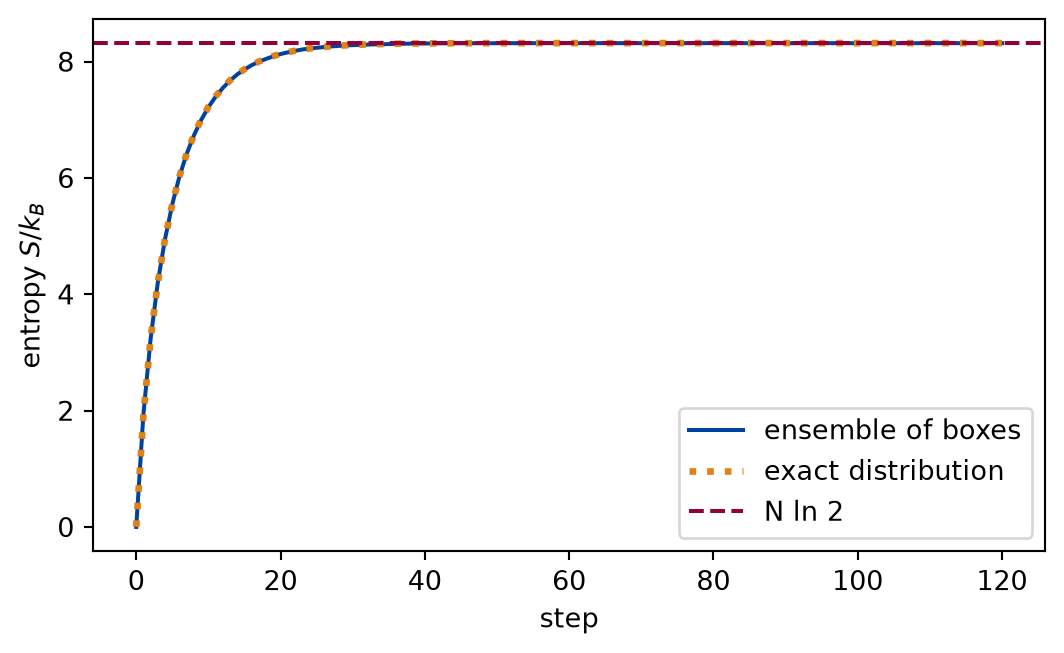
Six runs of an ensemble of five thousand boxes of twelve particles, each started with every particle on the left. The ensemble entropy is estimated from the observed frequencies at every step, and compared with the entropy of the exact distribution of the model.

MEMBERS = 5000
STEPS = 120
SEEDS = range(6)

src/pbc/thermodynamics/experiments/entropy_from_ensembles.py, lines 39 to 41, read from the repository when this page was built.

def ensemble_runs(experiment: Experiment):
    """Six runs of an ensemble of boxes from all particles on the left: the
    entropy of the ensemble at every step against that of the exact
    distribution; record the table of four steps."""
    runs = [
        ehrenfest_ensemble(N, MEMBERS, STEPS, np.random.default_rng(seed))
        for seed in SEEDS
    ]
    estimates = np.array(
        [[gibbs_entropy(distribution(row, N), N) for row in counts] for counts in runs]
    )
    exact_rows = exact_distribution(N, N, STEPS)
    exact_entropy = np.array([gibbs_entropy(row, N) for row in exact_rows])
    mean_estimate = estimates.mean(axis=0)

    checkpoints = [0, 10, 30, 120]
    experiment.table(
        "ensemble-runs",
        [
            (t, mean_estimate[t], exact_entropy[t], equilibrium_entropy(N))
            for t in checkpoints
        ],
        [
            ("step", "", "d"),
            ("entropy of the ensemble", "", ".3f"),
            ("entropy of the exact distribution", "", ".3f"),
            ("N ln 2", "", ".3f"),
        ],
        "The entropy S / k_B of the ensemble averaged over six runs, that of the "
        "exact distribution of the model, and the equilibrium value, at four "
        "steps.",
    )
    return runs, mean_estimate, exact_entropy

src/pbc/thermodynamics/experiments/entropy_from_ensembles.py, lines 94 to 126, read from the repository when this page was built.

The entropy S / k_B of the ensemble averaged over six runs, that of the exact distribution of the model, and the equilibrium value, at four steps.
step	entropy of the ensemble	entropy of the exact distribution	N ln 2
0	0.000	0.000	8.318
10	7.215	7.221	8.318
30	8.283	8.285	8.318
120	8.316	8.318	8.318

def draw_entropy_growth(mean_estimate, exact_entropy) -> Figure:
    """The entropy of the ensemble and of the exact distribution against the
    step."""
    fig, ax = plt.subplots(figsize=(6.4, 3.6))
    steps = np.arange(STEPS + 1)
    ax.plot(steps, mean_estimate, color="#00429d", label="ensemble of boxes")
    ax.plot(
        steps,
        exact_entropy,
        color="#e08214",
        linestyle=":",
        linewidth=2.5,
        label="exact distribution",
    )
    ax.axhline(equilibrium_entropy(N), color="#93003a", linestyle="--", label="N ln 2")
    ax.set_xlabel("step")
    ax.set_ylabel(r"entropy $S/k_B$")
    ax.legend()
    return fig

src/pbc/thermodynamics/experiments/entropy_from_ensembles.py, lines 129 to 147, read from the repository when this page was built.

Line plot of the entropy in units of the Boltzmann constant against the step. A solid curve rises from zero, steeply at first and then more slowly, and flattens at a horizontal dashed line, with a dotted curve of the exact distribution on top of it. — Figure 1: simulated The entropy of the ensemble starts at zero, because every box is in the same microstate, rises as the boxes spread over the macrostates, and levels off at the logarithm of all microstates. The estimate follows the exact curve.

The ensemble starts in one microstate and its entropy is zero. The model moves it towards the equilibrium and the entropy rises towards $N\ln 2$ , along the curve of the exact distribution, which does not decrease at any step.

def mean_check(experiment: Experiment, runs) -> float:
    """The mean number of particles on the left over six runs against the
    exact formula; record the table and return the largest distance in
    standard errors."""
    steps = np.arange(STEPS + 1)
    exact_mean = mean_left(N, N, steps)
    mean_runs = np.array([counts.mean(axis=1) for counts in runs])
    mean_value = mean_runs.mean(axis=0)
    mean_error = mean_runs.std(axis=0, ddof=1) / np.sqrt(len(runs))
    mean_checkpoints = [10, 30, 60, 120]
    experiment.table(
        "mean-check",
        [
            (
                t,
                mean_value[t],
                mean_error[t],
                exact_mean[t],
                abs(mean_value[t] - exact_mean[t]) / mean_error[t],
            )
            for t in mean_checkpoints
        ],
        [
            ("step", "", "d"),
            ("mean number on the left", "", ".3f"),
            ("standard error", "", ".3f"),
            ("exact mean", "", ".3f"),
            ("difference", "standard errors", ".1f"),
        ],
        "The mean number of particles on the left over six runs at four steps, "
        "against the exact formula.",
    )
    return max(
        abs(mean_value[t] - exact_mean[t]) / mean_error[t] for t in mean_checkpoints
    )

src/pbc/thermodynamics/experiments/entropy_from_ensembles.py, lines 150 to 184, read from the repository when this page was built.

The mean number of particles on the left over six runs at four steps, against the exact formula.
step	mean number on the left	standard error	exact mean	difference (standard errors)
10	8.518	0.005	8.513	0.9
30	6.448	0.010	6.441	0.7
60	6.018	0.014	6.032	1.1
120	6.011	0.007	6.000	1.5

Numerically verified (twelve particles, five thousand boxes per run, six runs, four standard errors): The mean number of particles on the left follows $N/2 + (n_0 - N/2)(1 - 1/N)^t$ within four standard errors at the four steps shown. The largest difference is 1.5 standard errors.

The entropy at equilibrium and what a finite ensemble can show

After many steps every box is at equilibrium and the entropy of the ensemble should be $N\ln 2$ . The plug-in estimate falls short of it; the question is by how much, and whether the shortfall is the one the correction predicts.

LATE = 12 * N

src/pbc/thermodynamics/experiments/entropy_from_ensembles.py, line 44, read from the repository when this page was built.

def equilibrium_check(experiment: Experiment) -> list:
    """The equilibrium entropy estimated from ensembles of three sizes,
    before and after the correction of the bias; record the table and return
    its rows."""
    rows = []
    for members in (200, 2000, 20000):
        raw, corrected = [], []
        for seed in SEEDS:
            counts = ehrenfest_ensemble(N, members, LATE, np.random.default_rng(seed))
            p = distribution(counts[-1], N)
            raw.append(gibbs_entropy(p, N))
            corrected.append(raw[-1] + plug_in_bias(p, members))
        raw_mean, raw_error = mean_and_error(np.array(raw))
        corrected_mean, corrected_error = mean_and_error(np.array(corrected))
        target = equilibrium_entropy(N)
        rows.append(
            (
                members,
                target - raw_mean,
                abs(raw_mean - target) / raw_error,
                abs(corrected_mean - target) / corrected_error,
            )
        )

    experiment.table(
        "equilibrium-check",
        rows,
        [
            ("boxes per run", "", "d"),
            ("shortfall of the plug-in estimate", "", ".5f"),
            ("plug-in estimate off by", "standard errors", ".1f"),
            ("corrected estimate off by", "standard errors", ".1f"),
        ],
        "The equilibrium entropy of the ensemble estimated from six runs of three "
        "sizes, as a shortfall from N ln 2 and in standard errors, before and "
        "after the first-order correction of the bias.",
    )
    return rows

src/pbc/thermodynamics/experiments/entropy_from_ensembles.py, lines 187 to 224, read from the repository when this page was built.

The equilibrium entropy of the ensemble estimated from six runs of three sizes, as a shortfall from N ln 2 and in standard errors, before and after the first-order correction of the bias.
boxes per run	shortfall of the plug-in estimate	plug-in estimate off by (standard errors)	corrected estimate off by (standard errors)
200	0.04000	6.1	2.8
2000	0.00304	7.7	0.8
20000	0.00029	13.7	0.5

Numerically verified (twelve particles, six runs, four standard errors, bias corrected to first order): At equilibrium the entropy of the ensemble, estimated from the observed frequencies with the first-order correction of the bias, agrees with $N\ln 2$ within four standard errors at three sizes of ensemble. The corrected estimate is off by at most 2.8 standard errors. The plug-in estimate alone is off by 14 standard errors at the largest size: its shortfall shrinks as the ensemble grows, from 0.040 to 0.00029, but its standard error shrinks as fast, because the entropy is at its maximum, where the first-order fluctuations of the frequencies drop out. The shortfall therefore stays many standard errors long and has to be corrected, not averaged away.

Limits

A closed form for a toy model. The check compares a computed entropy with $N\ln 2$ , the entropy of two halves and distinguishable particles. It shows that the program computes the entropy of the ensemble it is given. It does not show that a gas has this entropy, and it contains no measurement.
The estimate is biased. An entropy computed from frequencies is low, by an amount the lesson estimates to first order. For an ensemble that is small against the number of macrostates, or one with macrostates seen once, the correction is not reliable. A larger $N$ at the same number of boxes makes this worse.
A shuffle is not Newton’s laws. The entropy of this model rises because its dynamics is a random shuffle with a uniform equilibrium. For a system with deterministic, reversible laws the rise of the entropy of a coarse description needs the further argument of the coarse-graining, and the model does not address it.
Recurrence. With twelve particles the ensemble returns to a state with all particles on the left every few thousand steps on average, so the model does not forbid the reverse of the spreading, it makes it rare. The odds fall as $2^{-N}$ , so for a mole of particles the return is not seen in any time.
Two halves, not a gas. Mixing, temperature, and heat are not part of the model.

Self-check. In a run, the entropy of one box is always zero, because a box is always in one microstate. Why does the entropy of the ensemble still rise?

Because each box’s microstate gets more complicated as the particles spread.

No. A box is in a single microstate at every step, with no entropy of its own. The model has no complexity of a microstate to measure.
Because the entropy belongs to the distribution of the boxes over microstates, and that distribution spreads out.

Right. At the start every box is in the same microstate, so the distribution is concentrated and the entropy is zero. The shuffle makes the boxes differ, and the entropy of what is known about a box falls to that of equal chances at equilibrium.

Solution to the self-check

The entropy of this lesson is a property of an ensemble, or of what an observer knows about the microstate. The shuffle spreads the boxes over microstates, so the observer knows less and the entropy is larger. That is also why the entropy estimate needs many boxes: one box has no distribution.

Exercises

Exercise 1. How many boxes. The shortfall of the plug-in estimate at equilibrium is about $(K-1)/(2M)$ with $K = N+1$ . How many boxes make it smaller than a thousandth for twelve particles, and is it?

Hint 1 of 1 for exercise 1

Solve the bias formula for the number of boxes.

Solution to exercise 1

$M > N/(2\times 10^{-3})$ , so six thousand boxes at least.

def boxes_for_a_thousandth(experiment: Experiment) -> None:
    """Exercise 1: the number of boxes for a shortfall of a thousandth, and
    the shortfall measured with it; record the table."""
    needed = int(np.ceil(N / (2 * 1e-3)))
    shortfalls = []
    for seed in SEEDS:
        counts = ehrenfest_ensemble(N, needed, LATE, np.random.default_rng(seed))
        shortfalls.append(
            equilibrium_entropy(N) - gibbs_entropy(distribution(counts[-1], N), N)
        )
    experiment.table(
        "boxes-for-a-thousandth",
        [(needed, float(np.mean(shortfalls)))],
        [("boxes", "", "d"), ("mean shortfall", "", ".5f")],
        "The number of boxes the formula asks for and the shortfall of the plug-in "
        "estimate measured with it, over six runs.",
    )

src/pbc/thermodynamics/experiments/entropy_from_ensembles.py, lines 227 to 243, read from the repository when this page was built.

The number of boxes the formula asks for and the shortfall of the plug-in estimate measured with it, over six runs.
boxes	mean shortfall
6000	0.00090

The shortfall is of the size asked for.

Exercise 2. More particles. The ensemble of forty particles starts with all of them on the left. How many steps does the mean number on the left need to come within one particle of $N/2$ , and how many does the exact formula give?

Solution to exercise 2

The distance from $N/2$ falls as $(1-1/N)^t$ , so it is one particle after $t = \ln(N/2)/(-\ln(1-1/N))$ steps.

def approach_to_the_middle(experiment: Experiment) -> None:
    """Exercise 2: the steps for the mean of forty particles to come within
    one of the middle, by the formula and in one ensemble; record the
    table."""
    n_big = 40
    t_formula = np.log(n_big / 2) / -np.log(1 - 1 / n_big)
    big = ehrenfest_ensemble(n_big, 4000, 200, np.random.default_rng(0))
    distance = np.abs(big.mean(axis=1) - n_big / 2)
    t_measured = int(np.argmax(distance < 1.0))
    experiment.table(
        "approach-to-the-middle",
        [(t_formula, t_measured)],
        [("steps by the formula", "", ".1f"), ("steps in the ensemble", "", "d")],
        "The number of steps for the mean to come within one particle of N / 2, by "
        "the formula and in one ensemble.",
    )

src/pbc/thermodynamics/experiments/entropy_from_ensembles.py, lines 246 to 261, read from the repository when this page was built.

The number of steps for the mean to come within one particle of N / 2, by the formula and in one ensemble.
steps by the formula	steps in the ensemble
118.3	121

Run this experiment

This page was built from commit 6417e2ff90258bd2d2ba21d217eb7666fd24f680 of the repository.

In a clone at that commit, with the project’s Python packages installed, this command runs the experiment of this page:

uv run --locked --no-dev python -m pbc.thermodynamics.experiments.entropy_from_ensembles results

Files, tests, and every command

The files behind it:

site/lessons/thermodynamics/03-entropy-from-ensembles/index.qmd: this page, with every code cell.
src/pbc/thermodynamics/entropy.py: code the experiment runs.
src/pbc/thermodynamics/experiments/entropy_from_ensembles.py: code the experiment runs.
src/pbc/experiment.py: code the experiment runs.
tests/unit/test_thermodynamics.py: tests of that code.
tests/unit/test_entropy_from_ensembles_experiment.py: tests of that code.

With Git and uv installed (see the setup page), run:

git clone https://github.com/taspinar/physics-by-construction.git
cd physics-by-construction
git checkout 6417e2ff90258bd2d2ba21d217eb7666fd24f680
uv sync --locked --no-dev
uv run --locked --no-dev python -m pbc.thermodynamics.experiments.entropy_from_ensembles results

The experiment writes every figure of this page into results/, as <label>.png, and every number and table of the page, as the page shows it, into results/results.json. Its numbers match this page to the digits shown, and its figure files are the ones the page shows; digits beyond those can differ between machines, because floating-point libraries differ. Change the code of the experiment and run it again to see what changes.