Symbolic regression: a law from simulated data

An exhaustive search over power laws finds the period of a pendulum in simulated measurements, checks it on pendulums it never saw, and shows when the data cannot single out the law and at what noise the search stops finding it.

Course

Classical mechanics, lesson 22 of 31

Slot

D7, number 7 of the 13 slots of the path Scientific law discovery

Methods

Simulation

Difficulty

Advanced, level 3 of 3

What you’ll learn

Search a stated grammar of formulas for the simplest one that the data cannot reject, and say why the simplest
Test a recovered formula on held-out cases and state the range in which it holds
Recognise when several formulas describe the same observations, and name the measurement or the prior knowledge that separates them
Predict the noise at which a search loses a term of the law, and check the prediction over seeded repetitions

Prerequisites

Energy conservation, Inverse physics: parameters from observations.

Before you begin

Logarithms: the logarithm of a product and of a power
Statistics: least squares and the chi-square of residuals

Related

none

Previous

Unlearning a familiar law: a modified force

Next

Discovering differential equations from trajectories

With scripts, this page keeps a record in your browser of whether you completed the lesson. Nothing is stored without them.

With scripts, this place suggests what to do next, with the reason, from the progress saved in your browser. Without them, follow the learning path.

The inverse-physics lesson started from a model and asked for its parameters. Here the model itself is unknown. A table of measurements, the period of a pendulum next to its length, the gravity it swings in, its mass, and the angle it was released from, should be turned into a formula that a person can read. That is symbolic regression: a search over formulas rather than over the numbers in one formula.

The question sounds easy because we know the answer, $T = 2\pi\sqrt{L/g}$ . That is exactly why it is a good first case. A method that cannot find a law we know from data we made has no business being trusted with a law we do not know. And even here the honest answers are more interesting than “found it”: the formula holds only where the data were taken, the data sometimes cannot tell two formulas apart, and noise removes terms in a way that can be predicted in advance.

No language model is used in this lesson. The search is a plain program that tries every formula of a stated grammar. It is the baseline that the later discovery lessons, with or without an agent, are compared with.

Assumptions

The measurements come from a simulation. Each period is the time a simulated pendulum (pbc.mechanics.pendulum, integrated with the fourth-order Runge-Kutta method) takes to swing out and back. If the simulation were wrong, the search would faithfully find the wrong law; the page checks the simulated periods against the exact period first.
The law is a power law of the variables. The grammar holds the products $c\,L^{p_1} g^{p_2} m^{p_3} \theta_0^{p_4}$ with every exponent on the half-integers from $-2$ to $2$ . A law of another shape cannot be found, only approximated; the search then says that no form fits.
The noise is relative, Gaussian in the logarithm, and known. The search judges a form by its chi-square at the stated noise. If the stated noise is too small, every form is rejected; if it is too large, wrong forms pass.
Simpler is chosen, not proved. Among the forms the data do not reject, the search picks the one with the fewest variables and the smallest exponents. That is a rule of the method. The data only say which forms are rejected.
The probed ranges are the domain of the result. Lengths, gravities, masses, and amplitudes are drawn within fixed ranges. A formula found there is a statement about that region.

A grammar, a fit, and a rule for choosing

The data

LENGTHS = (0.2, 2.0)  # m
GRAVITIES = (1.6, 25.0)  # m/s², from the Moon to Jupiter
MASSES = (0.1, 2.0)  # kg
AMPLITUDES = (0.02, 0.1)  # rad
SAMPLES = 24
RESOLUTION = 1e-3  # the relative resolution of a period without added noise
SEED = 0

src/pbc/mechanics/experiments/symbolic_regression.py, lines 29 to 35, read from the repository when this page was built.

def simulated_period(
    length: float, gravity: float, mass: float, amplitude: float
) -> float:
    """The period in s of a pendulum released from rest at ``amplitude``
    (rad), simulated with the fourth-order Runge-Kutta method at 400 steps
    per small-angle period: twice the time until the bob is at rest on the
    other side, where its velocity changes sign."""
    acceleration = newton(mass, pendulum_force(mass, length, gravity))
    steps = 400
    dt = 2 * np.pi * np.sqrt(length / gravity) / steps
    motion = simulate(
        State(0.0, [length * amplitude], [0.0]),
        acceleration,
        dt,
        4 * steps,
        step=rk4_step,
        until=lambda state: state.v[0] > 0,
    )
    v_before, v_after = motion.v[-2, 0], motion.v[-1, 0]
    half_period = motion.t[-2] + dt * v_before / (v_before - v_after)
    return float(2 * half_period)

src/pbc/mechanics/experiments/symbolic_regression.py, lines 58 to 78, read from the repository when this page was built.

The simulated periods of the 24 pendulums agree with the exact period, a complete elliptic integral of the amplitude, to a relative difference below 2e-08. That is far below the stated resolution, so the search sees the pendulum and not the integrator.

Every form of the grammar

Take logarithms, and every power law becomes a straight line: $\begin{aligned}\ln T = \ln c &+ p_1 \ln L + p_2 \ln g \\ &+ p_3 \ln m + p_4 \ln \theta_0.\end{aligned}$ For given exponents the best constant is the mean of what is left of $\ln T$ , and the chi-square is the sum of the squared remainders over the noise squared. Nothing has to be optimised, so the search can try all 6561 forms and miss none.

def power_law_search(
    variables: Mapping[str, ArrayLike],
    y: ArrayLike,
    sigma: float,
    exponents: Sequence[float] = HALF_STEPS,
) -> Search:
    """Fit every power law of ``variables`` to ``y``.

    ``variables`` maps a name to its positive values, one per measurement;
    ``y`` holds the positive measurements, with a relative noise of standard
    deviation ``sigma`` (the standard deviation of ``ln y``). Each variable
    takes each exponent of ``exponents``."""
    names = tuple(variables)
    logs = np.column_stack([np.log(np.asarray(variables[n], float)) for n in names])
    log_y = np.log(np.asarray(y, float))
    if sigma <= 0:
        raise ValueError(f"sigma must be positive, got {sigma}")
    if len(log_y) < 2:
        raise ValueError("a search needs at least two measurements")
    grid = np.array(list(itertools.product(exponents, repeat=len(names))), float)
    # In logarithms each form is a straight line: the constant is the mean of
    # what the exponents leave of ln y, and the rest is the misfit.
    residual = log_y[:, None] - logs @ grid.T
    log_c = residual.mean(axis=0)
    chi2 = ((residual - log_c) ** 2).sum(axis=0) / sigma**2
    unsorted = Search(names, grid, np.exp(log_c), chi2, len(log_y) - 1, sigma)
    order = np.lexsort((unsorted.complexity, chi2))
    return Search(
        names, grid[order], np.exp(log_c[order]), chi2[order], len(log_y) - 1, sigma
    )

src/pbc/discovery/symbolic.py, lines 161 to 190, read from the repository when this page was built.

A form is consistent when its chi-square is what the noise alone would give: at most the number of degrees of freedom plus three standard deviations of the chi-square distribution, here 43.3 for 23 degrees of freedom. Among the consistent forms the search chooses the simplest by its complexity, the number of variables the form uses plus the number of half steps in its exponents. The square root of $L/g$ has complexity four; $L$ alone, three.

What the search finds on clean data

TRUE_SHAPE = (0.5, -0.5, 0.0, 0.0)  # L^(1/2) g^(-1/2): the small-angle law
TOLERANCE = 0.005  # relative, on the constant 2 pi

src/pbc/mechanics/experiments/symbolic_regression.py, lines 38 to 39, read from the repository when this page was built.

def clean_search(experiment: Experiment) -> tuple[dict, np.ndarray, Search]:
    """The search on the clean periods; record the best form of each
    complexity."""
    variables, periods = pendulums()
    search = power_law_search(variables, periods, RESOLUTION)
    experiment.table(
        "pareto",
        [
            (
                f.complexity,
                f.formula(),
                f.chi2,
                "yes" if f.chi2 <= search.limit else "no",
            )
            for f in search.pareto()
        ],
        columns=[
            ("complexity", "", "d"),
            ("best form (period in s)", "", "s"),
            ("chi-square", "", ".3g"),
            ("consistent", "", "s"),
        ],
        caption="The best power law of each complexity on the clean periods, with"
        " the chi-square at the stated resolution, to three significant digits.",
    )
    return variables, periods, search

src/pbc/mechanics/experiments/symbolic_regression.py, lines 114 to 139, read from the repository when this page was built.

The best power law of each complexity on the clean periods, with the chi-square at the stated resolution, to three significant digits.
complexity	best form (period in s)	chi-square	consistent
0	1.57	5e+06	no
2	1.691 L^(1/2)	1.04e+06	no
4	6.286 L^(1/2) g^(-1/2)	0.805	yes

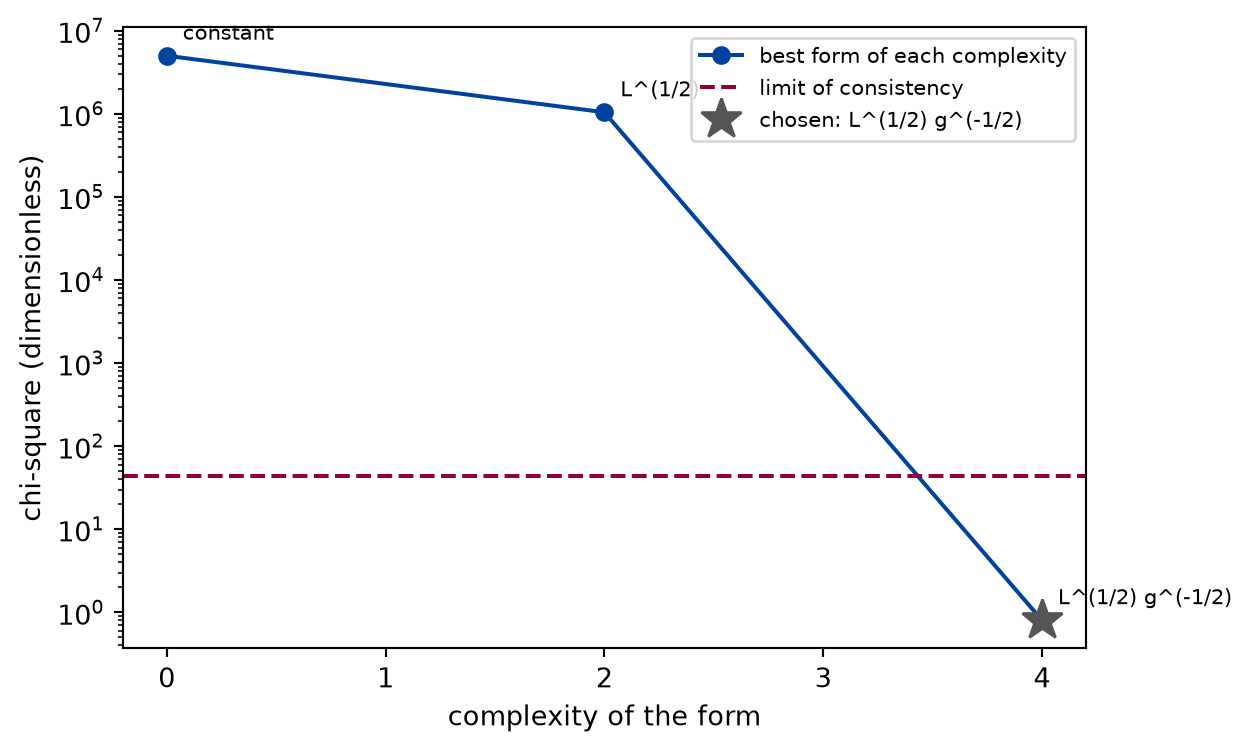
The table is the Pareto front: for each complexity, the best form, kept only if it fits better than every simpler one. A constant period is far off, a period that grows as the square root of the length is better but still rejected, and the next step, dividing by the square root of the gravity, drops the chi-square below the limit. Of all 6561 forms, 1 is consistent.

def draw_pareto(search: Search) -> Figure:
    """The best chi-square of each complexity, the limit of consistency, and
    the chosen form."""
    fig, ax = plt.subplots(figsize=(6.4, 3.8), constrained_layout=True)
    front = search.pareto()
    ax.semilogy(
        [f.complexity for f in front],
        [f.chi2 for f in front],
        color=FIGURE_COLOURS[0],
        marker="o",
        linestyle="-",
        label="best form of each complexity",
    )
    ax.axhline(
        search.limit,
        color=FIGURE_COLOURS[1],
        linestyle="--",
        label="limit of consistency",
    )
    chosen = search.chosen
    ax.semilogy(
        [chosen.complexity],
        [chosen.chi2],
        linestyle="none",
        marker="*",
        markersize=16,
        color=FIGURE_COLOURS[2],
        label="chosen: " + chosen.shape,
    )
    for form in front:
        ax.annotate(
            "constant" if form.shape == "1" else form.shape,
            (form.complexity, form.chi2),
            textcoords="offset points",
            xytext=(6, 6),
            fontsize=8,
        )
    ax.set_xticks(range(max(f.complexity for f in front) + 1))
    ax.set_xlabel("complexity of the form")
    ax.set_ylabel("chi-square (dimensionless)")
    ax.legend(loc="upper right", fontsize=8)
    return fig

src/pbc/mechanics/experiments/symbolic_regression.py, lines 287 to 328, read from the repository when this page was built.

Line plot with markers on a logarithmic vertical axis of chi-square against the complexity of the form. The points fall steeply from left to right: a constant at the top, the square root of the length below it, and the small-angle law, marked with a star, far below. A dashed horizontal line, the limit of consistency, lies between the last two points. — Figure 1: simulated The best power law of each complexity on the clean periods. The chi-square falls by orders of magnitude as the square root of the length and then of the gravity enter, and only the small-angle law lies below the limit of consistency (dashed).

Numerically verified (simulated pendulums in the probed ranges, power laws with half-integer exponents, relative resolution 0.1 percent): The search chooses 6.286 L^(1/2) g^(-1/2) from the clean periods, the small-angle law with a constant of 6.2855 against $2\pi =$ 6.2832, an error of 0.04 percent within the tolerance of 0.5 percent: the law is recovered. The mass and the amplitude are left out because no form with them fits better. The constant is a little above $2\pi$ , and not by chance: the pendulums swing at small but finite amplitudes, and a finite amplitude makes the period slightly longer. The correction is smaller than the resolution, so the search cannot see it as a term, but it can see it in the constant.

The program

The search itself is the one excerpt above. Its result, a Search, turns the fitted forms into statements about the data: the consistent forms, the rivals of the chosen one, and the Pareto front, which is the trade-off the choice was made on. A helper gives the noise at which a given form stops being rejected, which the section on noise uses.

@dataclass(frozen=True)
class Search:
    """The outcome of a search over the grammar: every form, fitted, as one
    row of arrays per form, best chi-square first.

    ``chosen`` is the simplest consistent form, or ``None`` with the
    ``reason``; ``rivals`` are the consistent forms whose chi-square is within
    ``TIE`` of the best one: forms the data cannot tell apart from it."""

    names: tuple[str, ...]
    exponents: Array  # one row per form, one column per variable
    constants: Array
    chi2: Array
    dof: int
    sigma: float

    def form(self, index: int) -> PowerLaw:
        """The form of row ``index``."""
        return PowerLaw(
            self.names,
            tuple(map(float, self.exponents[index])),
            float(self.constants[index]),
            float(self.chi2[index]),
        )

    @cached_property
    def forms(self) -> tuple[PowerLaw, ...]:
        return tuple(self.form(i) for i in range(len(self.chi2)))

    @property
    def limit(self) -> float:
        """The largest chi-square that counts as consistent: the rule of
        ``pbc.discovery.baselines.consistent``."""
        return self.dof + FIT_SIGMAS * math.sqrt(2 * self.dof)

    @property
    def complexity(self) -> NDArray[np.int64]:
        """The complexity of each form, as ``PowerLaw.complexity``."""
        steps = np.rint(np.abs(2 * self.exponents)).astype(int)
        return (self.exponents != 0).sum(axis=1) + steps.sum(axis=1)

    def _consistent(self) -> NDArray[np.intp]:
        return np.flatnonzero(self.chi2 <= self.limit)

    def consistent(self) -> tuple[PowerLaw, ...]:
        return tuple(self.form(i) for i in self._consistent())

    @property
    def chosen(self) -> PowerLaw | None:
        good = self._consistent()
        if not good.size:
            return None
        # The rows are in order of chi-square, so the first of the simplest
        # is the best fit among them.
        return self.form(good[np.argmin(self.complexity[good])])

    @property
    def rivals(self) -> tuple[PowerLaw, ...]:
        good = self._consistent()
        return tuple(self.form(i) for i in good if self.chi2[i] <= self.chi2[0] + TIE)

    @property
    def reason(self) -> str:
        if self.chosen is not None:
            return ""
        return (
            "no form of the grammar is consistent: the best has a chi-square of"
            f" {self.chi2[0]:.3g} for {self.dof} degrees of freedom"
        )

    def pareto(self) -> tuple[PowerLaw, ...]:
        """The best form of each complexity that beats every simpler one:
        the trade-off between simplicity and fit."""
        front: list[PowerLaw] = []
        for i in np.lexsort((self.chi2, self.complexity)):
            if not front or self.chi2[i] < front[-1].chi2:
                front.append(self.form(i))
        return tuple(front)

src/pbc/discovery/symbolic.py, lines 81 to 158, read from the repository when this page was built.

def noise_floor(search: Search, form: PowerLaw) -> float:
    """The relative noise at which ``form``, fitted by ``search`` on data with
    no noise beyond ``search.sigma``, is expected to become consistent.

    The misfit of the form grows its chi-square by ``form.chi2`` at the noise
    ``search.sigma``, and by that times ``(search.sigma / s)**2`` at a noise
    ``s``; the noise itself adds one per degree of freedom on average. The
    form passes once the misfit is below the margin of the limit,
    ``FIT_SIGMAS * sqrt(2 * dof)``: below this noise the data reject the
    form, above it they cannot."""
    margin = FIT_SIGMAS * math.sqrt(2 * search.dof)
    return search.sigma * math.sqrt(form.chi2 / margin)

src/pbc/discovery/symbolic.py, lines 193 to 204, read from the repository when this page was built.

Worked examples

Held-out pendulums

A formula found in a region is tested outside it. The held-out pendulums are longer than any probed one, swing in a gravity not drawn, or are released far higher.

HELD_OUT = (  # length (m), gravity (m/s²), amplitude (rad)
    (5.0, 9.81, 0.05),
    (20.0, 3.7, 0.05),
    (1.0, 9.81, 0.3),
    (1.0, 9.81, 0.8),
    (1.0, 9.81, 1.5),
)

src/pbc/mechanics/experiments/symbolic_regression.py, lines 42 to 48, read from the repository when this page was built.

def held_out(experiment: Experiment, form: PowerLaw) -> list[float]:
    """The chosen form against pendulums outside the probed ranges; record
    the table and return the relative errors."""
    rows, errors = [], []
    for length, gravity, amplitude in HELD_OUT:
        period = simulated_period(length, gravity, 1.0, amplitude)
        predicted = float(
            form.predict({"L": length, "g": gravity, "m": 1.0, "theta0": amplitude})
        )
        errors.append(predicted / period - 1)
        rows.append((length, gravity, amplitude, period, predicted, 100 * errors[-1]))
    experiment.table(
        "held-out",
        rows,
        columns=[
            ("length", "m", "g"),
            ("gravity", "m/s²", "g"),
            ("amplitude", "rad", "g"),
            ("simulated period", "s", ".4f"),
            ("predicted period", "s", ".4f"),
            ("error", "%", ".2f"),
        ],
        caption="The chosen form on held-out pendulums of mass 1 kg: two outside"
        " the probed lengths and gravities at small amplitude, three at"
        " amplitudes beyond the probed ones. Periods to four decimals.",
    )
    return errors

src/pbc/mechanics/experiments/symbolic_regression.py, lines 154 to 180, read from the repository when this page was built.

The chosen form on held-out pendulums of mass 1 kg: two outside the probed lengths and gravities at small amplitude, three at amplitudes beyond the probed ones. Periods to four decimals.
length (m)	gravity (m/s²)	amplitude (rad)	simulated period (s)	predicted period (s)	error (%)
5	9.81	0.05	4.4864	4.4874	0.02
20	3.7	0.05	14.6104	14.6136	0.02
1	9.81	0.3	2.0174	2.0068	-0.53
1	9.81	0.8	2.0894	2.0068	-3.95
1	9.81	1.5	2.3310	2.0068	-13.91

Numerically verified (the held-out pendulums of the table): On the held-out pendulums at small amplitude the chosen form predicts the simulated period within 0.02 percent, also at lengths ten times the longest probed one; at an amplitude of $1.5$ rad it is off by 14 percent. The search found the law of small swings, which is all the data contained. Whether it is “the” law of the pendulum is not a question these data can answer: only data at large amplitude can, and there the formula fails.

Data that cannot single out the law

Suppose every pendulum swings on the Earth. The gravity is then the same in every row, and its exponent can be anything: whatever power of $g$ the form has, the constant absorbs it.

def earth_only(experiment: Experiment) -> tuple[Search, float]:
    """The search on pendulums that all swing at the gravity of the Earth;
    record the forms the data cannot tell apart, and return the search and
    the error of its choice on the Moon."""
    variables, periods = pendulums(gravities=(EARTH, EARTH))
    search = power_law_search(variables, periods, RESOLUTION)
    experiment.table(
        "earth-rivals",
        [
            (f.formula(), f.chi2)
            for f in sorted(search.rivals, key=lambda f: (f.complexity, f.exponents))
        ],
        columns=[("form (period in s)", "", "s"), ("chi-square", "", ".3f")],
        caption="Every form within one unit of chi-square of the best, on pendulums"
        " that all swing at the gravity of the Earth; chi-square to three decimals.",
    )
    moon = {"L": 1.0, "g": 1.62, "m": 1.0, "theta0": 0.05}
    period = simulated_period(1.0, 1.62, 1.0, 0.05)
    error = float(search.chosen.predict(moon)) / period - 1
    return search, error

src/pbc/mechanics/experiments/symbolic_regression.py, lines 183 to 202, read from the repository when this page was built.

Every form within one unit of chi-square of the best, on pendulums that all swing at the gravity of the Earth; chi-square to three decimals.
form (period in s)	chi-square
2.007 L^(1/2)	0.805
6.286 L^(1/2) g^(-1/2)	0.805
0.6409 L^(1/2) g^(1/2)	0.805
19.68 L^(1/2) g^(-1)	0.805
0.2047 L^(1/2) g	0.805
61.64 L^(1/2) g^(-3/2)	0.805
0.06536 L^(1/2) g^(3/2)	0.805
193 L^(1/2) g^(-2)	0.805
0.02087 L^(1/2) g^(2)	0.805

Numerically verified (power laws with half-integer exponents; simulated pendulums at one gravity): On pendulums that all swing at the gravity of the Earth, 9 forms, one for each exponent of the gravity in the grammar, fit with the same chi-square. The search chooses the simplest, 2.007 L^(1/2), which predicts the period of a pendulum on the Moon 59 percent too short. None of these forms is wrong about the data. The data do not contain the answer, and the choice of the simplest is a rule, not evidence. Two things separate the forms. A measurement: pendulums in other gravities, as in the first search. Or prior knowledge: the period is a time, and only the square root of $L/g$ makes a time out of a length and an acceleration. The first exercise applies that rule to the search.

A law outside the grammar is the other way to fail. With amplitudes up to $1.2$ rad, the period depends on the amplitude through an elliptic integral, which no power law follows:

def wide_amplitudes() -> Search:
    """The search on pendulums released at amplitudes up to 1.2 rad, where
    the period depends on the amplitude in a way no power law follows."""
    variables, periods = pendulums(amplitudes=WIDE_AMPLITUDES)
    return power_law_search(variables, periods, RESOLUTION)

src/pbc/mechanics/experiments/symbolic_regression.py, lines 205 to 209, read from the repository when this page was built.

The search reports: no form of the grammar is consistent: the best has a chi-square of 2.2e+04 for 23 degrees of freedom. The best form, 6.604 L^(1/2) g^(-1/2), is the small-angle law with a larger constant, an average over the amplitudes. The search does not offer it as a result, and neither should a reader.

Noise

Measured periods have noise. The search is run on noisy copies of the clean periods, each period multiplied by the exponential of a Gaussian draw, with the noise known to the search, at 7 levels and over 20 seeds each.

NOISE_LEVELS = (0.001, 0.01, 0.03, 0.1, 0.2, 0.3, 0.5)  # relative
SEEDS = 20

src/pbc/mechanics/experiments/symbolic_regression.py, lines 51 to 52, read from the repository when this page was built.

def noise_sweep(
    experiment: Experiment, variables: dict, periods: np.ndarray
) -> list[tuple[float, int, int, int]]:
    """The search at each noise level on ``SEEDS`` noisy copies of the clean
    periods; record how often it chooses the form of the law, how far its
    constant then is from 2 pi, and what it chooses otherwise."""
    outcomes = []
    rows = []
    for noise in NOISE_LEVELS:
        searches = [
            power_law_search(variables, noisy_periods(periods, noise, seed), noise)
            for seed in range(SEEDS)
        ]
        right = [s.chosen for s in searches if right_form(s)]
        empty = sum(s.chosen is None for s in searches)
        others = Counter(
            s.chosen.shape
            for s in searches
            if s.chosen is not None and not right_form(s)
        )
        wrong = sum(others.values())
        common = others.most_common(1)[0][0] if others else ""
        scatter = (
            100
            * float(
                np.sqrt(np.mean([(f.constant / (2 * np.pi) - 1) ** 2 for f in right]))
            )
            if right
            else None
        )
        outcomes.append((noise, len(right), wrong, empty))
        rows.append(
            (
                100 * noise,
                len(right),
                scatter,
                100 * noise / np.sqrt(SAMPLES),
                wrong,
                common,
            )
        )
    experiment.table(
        "noise-sweep",
        rows,
        columns=[
            ("noise", "%", "g"),
            (f"form of the law chosen (of {SEEDS})", "", "d"),
            ("error of its constant", "%", ".2f"),
            ("expected error of the constant", "%", ".2f"),
            ("another form chosen", "", "d"),
            ("most frequent other form", "", "s"),
        ],
        caption=f"The search on {SEEDS} noisy copies of the periods at each noise"
        " level, the noise known to the search. The error of the constant is the"
        " root-mean-square relative error of 2 pi over the copies where the form"
        " of the law was chosen; the expected error is the noise divided by the"
        " square root of the number of pendulums. Errors to two decimals.",
    )
    return outcomes

src/pbc/mechanics/experiments/symbolic_regression.py, lines 219 to 277, read from the repository when this page was built.

The search on 20 noisy copies of the periods at each noise level, the noise known to the search. The error of the constant is the root-mean-square relative error of 2 pi over the copies where the form of the law was chosen; the expected error is the noise divided by the square root of the number of pendulums. Errors to two decimals.
noise (%)	form of the law chosen (of 20)	error of its constant (%)	expected error of the constant (%)	another form chosen	most frequent other form
0.1	20	0.04	0.02	0
1	20	0.17	0.20	0
3	20	0.52	0.61	0
10	20	1.76	2.04	0
20	9	4.08	4.08	11	L^(1/2)
30	2	5.75	6.12	18	L^(1/2)
50	1	10.52	10.21	19	1

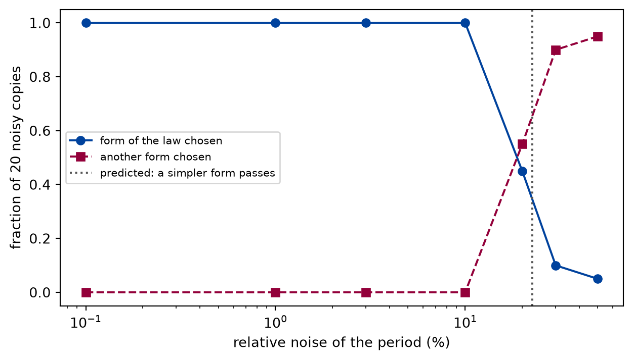
The failure can be predicted from the clean data. On them, the simplest rejected form, L^(1/2), misses by a fixed amount. A noise large enough to hide that misfit makes the form consistent, and once it is consistent the search prefers it, because it is simpler. The helper noise_floor turns the misfit into that noise: 23 percent.

def draw_noise_sweep(
    outcomes: list[tuple[float, int, int, int]], floor: float
) -> Figure:
    """How often the search chooses the form of the law, and how often
    another form, against the noise; the predicted level where a simpler form
    passes."""
    fig, ax = plt.subplots(figsize=(6.4, 3.6), constrained_layout=True)
    noise = [100 * o[0] for o in outcomes]
    ax.semilogx(
        noise,
        [o[1] / SEEDS for o in outcomes],
        color=FIGURE_COLOURS[0],
        marker="o",
        linestyle="-",
        label="form of the law chosen",
    )
    ax.semilogx(
        noise,
        [o[2] / SEEDS for o in outcomes],
        color=FIGURE_COLOURS[1],
        marker="s",
        linestyle="--",
        label="another form chosen",
    )
    ax.axvline(
        100 * floor,
        color=FIGURE_COLOURS[2],
        linestyle=":",
        label="predicted: a simpler form passes",
    )
    ax.set_xlabel("relative noise of the period (%)")
    ax.set_ylabel(f"fraction of {SEEDS} noisy copies")
    ax.set_ylim(-0.05, 1.05)
    ax.legend(loc="center left", fontsize=8)
    return fig

src/pbc/mechanics/experiments/symbolic_regression.py, lines 331 to 365, read from the repository when this page was built.

Line plot with markers of a fraction from zero to one against relative noise in percent on a logarithmic axis. The solid curve for the law stays at one for small noise and drops to near zero at the largest noise levels; the dashed curve for another form mirrors it, rising from zero. A dotted vertical line marks the predicted level, close to where the two curves cross. — Figure 2: simulated How often the search chooses the form of the small-angle law, and how often another form, against the noise of the period. The switch comes where the misfit of the simpler form drops below what the noise hides, close to the predicted level (dotted).

Numerically verified (these pendulums, twenty seeds per noise level, noise known to the search): The search chooses the form of the small-angle law on every noisy copy up to a noise of 10 percent, and loses the gravity at higher noise, where it prefers L^(1/2); the switch lies near the predicted level of 23 percent. Where the form is found, the error of its constant follows the noise divided by the square root of the number of pendulums. The failure is not a defect to tune away. A term of a law is visible only when its effect over the probed range is larger than what the noise hides; below that, a simpler formula describes the data as well, and choosing it is the honest reading. Wider ranges or more pendulums move the level, as the second exercise shows.

Limits

The grammar decides what can be found. Power laws with half-integer exponents contain the small-angle law. A search over a richer grammar (sums, functions of the variables) would have more forms that fit by chance, and the rule for choosing would matter even more.
Consistent is not true. A consistent form describes the data within the noise in the probed ranges. The held-out table shows where that holds; the large-amplitude row shows where it stops.
The choice of the simplest is a convention. The complexity counts variables and half steps; another count could prefer another form among consistent ones. Only where exactly one form is consistent does the rule not matter.
The noise is known and of one kind. The search uses the true noise. A noise that is underestimated rejects the law; one that is overestimated lets simpler forms in earlier. Systematic errors, such as a timer that runs fast, are not modelled.
One simulated system. The lesson recovers a law we already knew, from a simulation of it. It shows how the method behaves, not that it finds laws of nature from real measurements.

In plain words: the search finds the simplest formula that the data cannot reject. That is the law only as far as the data reach, and only when nothing simpler fits as well. Test it where it was not fitted, and know the noise at which it would have lost a term.

Self-check. Two forms fit a data set with the same chi-square, one with the gravity and one without. What does the search tell you, and what do you need to decide between them?

The simpler form is the law, because the search chose it.

The choice of the simplest is a rule of the method, not evidence. When the chi-square is the same, the data have no preference.
The data cannot tell them apart; a measurement that varies the gravity, or a constraint such as the units of the period, is needed.

Right. Equal chi-square means the observations carry no information about the term. A new measurement or prior knowledge has to supply it.
The form with the gravity, because the true law has it.

That is knowledge from outside the data. It is a valid reason only if it is stated as an assumption, as the units are in the first exercise.

Solution to the self-check

The search shows that the data do not determine the exponent of the gravity: the two forms are rivals. To decide, vary the gravity in the measurements, or add a constraint the data cannot supply, such as that the period has the units of a time.

Exercises

Exercise 1. Units as prior knowledge. Keep only the consistent forms of the search on the Earth that have the units of a time, with $L$ in metres, $g$ in metres per second squared, $m$ in kilograms, and the amplitude without a unit. How many are left, and which?

Hint 1 of 1 for exercise 1

A product of powers has the units of a time when the metres cancel, the seconds come out to the power one, and the kilograms cancel.

Solution to exercise 1

def units_filter(search: Search) -> list[PowerLaw]:
    """The consistent forms of ``search`` that have the units of a time:
    with L in m, g in m/s², m in kg, and the amplitude without a unit, the
    metres cancel when the exponents of L and g add to zero, the seconds
    remain when the exponent of g is -1/2, and the kilograms cancel when the
    exponent of m is zero."""
    return [
        f
        for f in search.consistent()
        if f.exponents[0] + f.exponents[1] == 0
        and f.exponents[1] == -0.5
        and f.exponents[2] == 0
    ]

src/pbc/mechanics/experiments/symbolic_regression.py, lines 368 to 380, read from the repository when this page was built.

1 form remains, 6.286 L^(1/2) g^(-1/2): the small-angle law with its constant. The units fixed the exponent of the gravity that the data could not, so the constant came out as $2\pi$ although every pendulum swung at the same gravity. This is the same information as pendulums on other planets, supplied as an assumption instead of a measurement.

Exercise 2. More pendulums. Repeat the noise sweep with four times as many pendulums, from 10 to 50 percent noise. Where does the search now lose the gravity, and by how much did the level move?

Hint 1 of 1 for exercise 2

The misfit of the simpler form is a sum over the pendulums, while the margin of the limit grows only as the square root of their number.

Solution to exercise 2

def more_samples(experiment: Experiment) -> None:
    """Exercise: the noise sweep with four times as many pendulums."""
    rng = np.random.default_rng(7)
    count = 4 * SAMPLES
    variables = {
        "L": rng.uniform(*LENGTHS, count),
        "g": rng.uniform(*GRAVITIES, count),
        "m": rng.uniform(*MASSES, count),
        "theta0": rng.uniform(*AMPLITUDES, count),
    }
    periods = np.array(
        [simulated_period(*p) for p in zip(*variables.values(), strict=True)]
    )
    rows = []
    for noise in (0.1, 0.2, 0.3, 0.5):
        hits = sum(
            right_form(
                power_law_search(variables, noisy_periods(periods, noise, s), noise)
            )
            for s in range(SEEDS)
        )
        rows.append((100 * noise, hits))
    experiment.table(
        "more-samples",
        rows,
        columns=[
            ("noise", "%", "g"),
            (f"form of the law chosen (of {SEEDS})", "", "d"),
        ],
        caption=f"The search on {count} pendulums instead of {SAMPLES}.",
    )

src/pbc/mechanics/experiments/symbolic_regression.py, lines 383 to 413, read from the repository when this page was built.

The search on 96 pendulums instead of 24.
noise (%)	form of the law chosen (of 20)
10	20
20	20
30	20
50	4

The law survives at noise levels where it was lost before. The misfit grows with the number of pendulums $n$ , the margin as $\sqrt{n}$ , so the noise floor grows as $n^{1/4}$ : four times the pendulums move it by a factor of about $\sqrt{2}$ , with the seeds adding scatter around that.

Run this experiment

This page was built from commit 3a83ab640162bf2b624c2b254d917ed5bdc7090d of the repository.

In a clone at that commit, with the project’s Python packages installed, this command runs the experiment of this page:

uv run --locked --no-dev python -m pbc.mechanics.experiments.symbolic_regression results

Files, tests, and every command

The files behind it:

site/lessons/agents-llm/08-symbolic-regression/index.qmd: this page, with every code cell.
src/pbc/discovery/symbolic.py: code the experiment runs.
src/pbc/discovery/baselines.py: code the experiment runs.
src/pbc/mechanics/pendulum.py: code the experiment runs.
src/pbc/mechanics/integrators.py: code the experiment runs.
src/pbc/mechanics/experiments/symbolic_regression.py: code the experiment runs.
src/pbc/experiment.py: code the experiment runs.
tests/unit/test_symbolic.py: tests of that code.
tests/unit/test_symbolic_regression_experiment.py: tests of that code.

With Git and uv installed (see the setup page), run:

git clone https://github.com/taspinar/physics-by-construction.git
cd physics-by-construction
git checkout 3a83ab640162bf2b624c2b254d917ed5bdc7090d
uv sync --locked --no-dev
uv run --locked --no-dev python -m pbc.mechanics.experiments.symbolic_regression results

The experiment writes every figure of this page into results/, as <label>.png, and every number and table of the page, as the page shows it, into results/results.json. Its numbers match this page to the digits shown, and its figure files are the ones the page shows; digits beyond those can differ between machines, because floating-point libraries differ. Change the code of the experiment and run it again to see what changes.